Forecasting
Forecasting.

Forecasting
E N D
Presentation Transcript
Should you carry an umbrella today? Part of the answer for you most likely depends on how much you care about getting wet! Assuming you care, then you have to look to the future and think about what you think might happen. You would be making a forecast, even if you have listened to the weather report. In a business setting we often can use a forecast as well. We might like to forecast sales, profit, the consumer price index, or units sold by a competitor. In a statistics class you may have seen how regression analysis can be used to forecast. I would like to start with an example and then go over some methods of forecasting.
Forecast Demand Table 11.3 has some demand data. Let’s start slowly with the example. Say demand in the first three periods was: Period Demand 1 10 2 18 3 29 The average of the demand in the 3 periods is (10 + 18 + 29)/3 = 57/3 = 19. This average can now be used as a forecast for the demand in period 4. This forecast will then help use decide how to schedule production.
Moving Average The idea behind the moving average method of forecasting is that next period will not be much different than the past few periods. In the example so far, I have waited three periods before I calculated an average. This would be called a three – period moving average method. On the next slide I continue with the example.
End of period 3 Period Demand Moving Average Forecast error=D-F 1 10 2 18 3 29 19 4 19 So, at the end of period 3 there is enough information to calculate a three-period moving average. At that point a forecast can be made for period 4. The forecast is that demand will be 19 and plans can be made accordingly. On the next slide let’s add the actual demand that happens in period 4 and show some other ideas.
Period 4 Period Demand Moving Average Forecast error=D-F 1 10 2 18 3 29 19 4 15 19 -4 With the passage of time and period 4 arriving we see demand actually is only 15. We planned on 19. This means we had an error of -4 when we take the actual minus the forecast. (I find this a bit weird because the -4 means we made too much!) Now, as we look to period 5 we can use the most recent 3 periods of actual data to calculate an average: (18 + 29 + 15) / 3 = 62/3 = 20.7. So at the end of period 4 we have the basis for the period 5 forecast. Let’s see that next.
Period 4 Period Demand Moving Average Forecast error=D-F 1 10 2 18 3 29 19 4 15 20.7 19 -4 5 20.7 So, at the end of period 4 we can 1) See how our forecast for period 4, called F4, was really the three-period moving average at period 3, called A3 (and thus F4 = A3), 2) See how good the forecast worked out by looking at the error D4 – F4, 3) Make a forecast for period 5 by using the three-period moving average up to period 4, F5 = A4.
Table row 13 As we look at the table on page 231 lets’ look at row 13 to make sure we understand what is happening. The forecast for period 13 is really the average of periods 10, 11, and 12. We do this at the end of period 12 and get 18.7. When actual demand comes in in period 13 we see the value 30 and we see the error = 30 – 18.7 = 11.3 The forecast for period 14 will be the average of periods 11, 12, and 13, for a value of 24.
Other moving averages In our example so far we have used a three-period moving average. We could have used a two-period, 4-period, or 10-period moving average. The advantage of using a longer time frame is that the new data point will have less influence and thus the forecasts from period to period will not change much, what is called stability. The disadvantage of using a longer time frame is that the forecasts are slow to respond to demand changes. Thus we could have persistent errors. Later we will go over ways to evaluate and choose methods of forecasting.
Weighted moving average In our example at the end of period 3 I calculated the average as (10 + 18 + 29)/3 = 57/3 = 19. By basic math rules I could have done the following (10 + 18 + 29)/3 = (1/3)10 + (1/3)18 + (1/3)29. The average you and I always calculate is really a weighted average where each data point is weighted the same, here 1/3. Some folks may want to give more weight to the most recent data point, and thus give less weight to less recent data points. This overcomes the problem of the forecast being slow to respond to demand changes. The requirement to use a weighted average is that each weight has to be between 0 and 1 and the sum of the weights has to add to 1.
Exponential Smoothing Exponential smoothing is another forecasting method. After some algebra, the method makes the forecast for next period = the forecast you had for this period plus a fraction of the error this period. In the book this is on page 233. The fraction is given the name of the small greek letter alpha, α. So, once you have the initial forecast and alpha, you are all set. Page 234 has a table with alpha = .1 and alpha = .3 and in both cases the initial forecast is 15 (an arbitrary number – though based on judgment). Note for period 2 the forecast when alpha = .1 is 14.5 = 15 + .1(-5), while for alpha = .3 the forecast is 13.5.
In general, the forecast error or deviation is defined as the actual value minus the forecast value. Say ei is the deviation for the ith unit, where units are time periods, and say di is the actual value and fi is the forecast value. Then ei = di – fi. In a data set when we have values for the actual data and forecasts, AD = Σ׀ei׀, or in words you take the absolute value of all the deviations, then add up the absolute values. A method of forecasting is called better if the method has a lower AD. This way the one with less error is chosen as better. If we divide the sum by n we get the mean absolute deviation of forecast errors, MAD.
Bias is another way to judge a forecasting method. Bias would just be to add up all the errors without taking the absolute value. This is also called CFE, or the cumulative sum of forecast errors. You would think that over time a method would have a bias of zero meaning some years you get positive errors and some years you get negative errors and the two cancel each other out. But, often we do not have the luxury of looking over a long period of time so we would say a method of forecasting is better if it has smaller bias. If a method has both smaller bias and smaller AD then it is preferred. But if one method has smaller bias but more error, then you have to decide which is the more desirable factor for you.
Tracking signal TS TS = CFE/MAD. If TS gets bigger than 6 or less than minus six, then the forecasting method should be stopped and reworked because we are too far off. Note the worked problems on pages 246, 247 and 248.

