Download

1 / 56
560 likes | 677 Vues
A Study of the Applicability of CFD to Knife Seal Design in the Gas Turbine Industry. Principal Advisors: Dr. Hasan Akay, IUPUI P. Chakka, PhD., Rolls-Royce T. Lambert, MS., Rolls-Royce. A Presentation to the Faculty of Purdue School of E&T, IUPUI

E N D
A Study of the Applicability of CFD to Knife Seal Design in the Gas Turbine Industry Principal Advisors: Dr. Hasan Akay, IUPUI P. Chakka, PhD., Rolls-Royce T. Lambert, MS., Rolls-Royce A Presentation to the Faculty of Purdue School of E&T, IUPUI by Joshua M. Peters in Partial Fulfillment of the Degree of Master of Science April 27, 2006
Note Numerical results, comparisons with test data, conclusions, and other information considered proprietary and/or sensitive have been removed from this presentation.
Outline Introduction Objective Numerical Method Computational Grids Description of Test Results and Validation Additional Studies Conclusions Acknowledgements References
Introduction • Knife/labyrinth seals are non-contact air seals used between rotating and non-rotating components where (air) leakage mass flow must be controlled or minimized.
Introduction (cont.) • Typical design practice: • Semi-empirical codes; interpolate/extrapolate test data. Results are valid inasmuch as new design is similar to tests. Right: Knife seal geometry and parameters assumed in typical seal design codes. Below: (Non)dimensional parameter characterizing mass flow rate thru seal.
Introduction (cont.) • Consequences of seal design error (grossly simplified): • Underprediction lower thrust/efficiency • Overprediction downstream overheating
Objective • Develop CFD model of a typical (single) knife seal for which test data exists; compare results and attempt to infer applicability of CFD to knife seal design.
Expected Computational Challenges Flow accelerates nearly 2 orders of magnitude in one knife height putting considerable demands on the solver and on the grid, particularly in the region of the knife tip. Flow is highly compressible at the knife tip and essentially incompressible in the balance of the flow. Sharp corners on knife create singularities in flowfield
Numerical Method Governing Equations Compressible Flow Equations Reynolds-Averaged N-S Turbulence Model Discretization Boundary Conditions Solver Method
0 0 0 0 0 Governing Equations1 Mass conservation: Momentum balance: …stress tensor:
0 0 0 Governing Equations Energy conservation: …where: …and sensible enthalpy for ideal gasses:
0 0 0 0 0 0 0 0 Governing Equations in Cylindrical Coordinates (2D) Mass conservation for compressible flow: Momentum balance, axial: Momentum balance, radial: …where:
Compressible Flow Physics Mach number and speed of sound: Relationship between static and stagnation conditions: Ideal gas law as implemented in FLUENT:
Governing Equations Reworked: RANS Variables decomposed into mean and fluctuating components: Resulting Reynolds averaged Navier-Stokes equations (interpreted, for compressible flows, as Favre-averaged):
Turbulence Model Spalart-Allmaras (1-Equation): Boussinesq hypothesis:
Discretization A conservation equation for an arbitrary CV: Discretized: …where: Linearized:
Segregated Solver Method (FLUENT) P*, rhou*, rhov* rho, u , v, P rhou* , rhov* P*, rhou*, rhov* …+ T*, v*, …
Boundary Conditions Operating Conditions: Pop=14.698psia Inlet: Total pressure (gauge; varied to control pressure ratio), total temperature (533R), hydraulic diameter and turbulence intensity (solution-based iterations) Outlet: Static pressure (gauge; fixed at 0 for all models), recirculation total temperature (533R) and modified turbulent viscosity (solution-based iterations)
Boundary Conditions (cont.) Stator (top): No-slip Knife/Disk: No-slip Rotor: No-slip or inviscid (<1% ΔW) Near-wall velocity profile: standard wall functions
Boundary Conditions (cont.) Turbulence intensity at inlet estimated by: Preliminary solutions were run with an estimated value; final solutions were obtained by iterating on density and velocity and updating turbulence intensity. Iterations were performed for modified turbulent viscosity at the outlet.
“Primary Grid” Characteristics: Quad, 26k cells, 40x50 at knife tip. Advantages: Reduced cell count, reduced aspect ratios near knife tip. Disadvantages: Slight increase in skewness near knife tip; non-stream-aligned faces. Below: Domain Left: Zoom on knife
“Primary Grid” (zoom) Above: Knife tip zoom. Maximum aspect ratio around 5.
“Secondary Grid” Characteristics: Quad BL, triangle 22k cells, 40x40 at knife tip Advantages: High resolution, locally-refined at knife tip, and extended outlet (hence smoothed outlet flow) improved convergence. Disadvantages: High aspect ratio and high skew in cells near knife tip. High resolution downstream of knife caused trouble for coupled solvers. Below: Computational domain Left: Zoom on center region
“Secondary Grid” (zoom) Above: Zoom on knife tip. 25% cell count reduction relative to “Primary Grid.” Mach number gradient based grid adaption applied, degrading already-poor convergence characteristics. Adaption not used in results presented.
2D Seal Rig (performed c.1970) (Removed. See slide #2, “Notes.”) Left: Labyrinth Seal Test Rig Below: Representative Single Knife Test (Removed. See slide #2, “Notes.”)
Rig Instrumentation Below: Labyrinth Seal Test Rig Instrumentation (Removed. See slide #2, “Notes.”)
Results and Validation 2D Planar Models vs. 2D Planar Test Data Axisymmetric Models vs. Semi-Empirical Codes Representative Residuals, Vectors, and Contour Plots
FLENT Model vs. Test – 2D Planar • Seven FLUENT models (planar) run at increasing pressure ratios: mass flow rate (W) in terms of the flow parameter Φ plotted versus pressure ratio. • Grid independence check @PR=2.0 using ‘Grid 3.’ (Removed. See slide #2, “Notes.”)
Model vs. Semi-Empirical Codes – Axisymmetric • Nine FLUENT models (axisymmetric) run at increasing pressure ratios: mass flow rate (W) in terms of the flow parameter Φ plotted versus pressure ratio. • Turbulence models compared at PR=3.0 (Removed. See slide #2, “Notes.”)
Model vs. Semi-Empirical Codes – Axisymmetric • Data from FLUENT (leading to plots). Iterative solution procedure: Density, velocity, and modified turbulent viscosity were obtained in solutions; turbulence intensity and modified turbulent viscosity were input as boundary conditions leading to new solutions and updated boundary conditions... (Removed. See slide #2, “Notes.”)
Typical Residuals and W Convergence at PR=2.00 Right: Scaled residuals thru 9000 iterations Below: Mass flow rate convergence (@ inlet) thru 9000 iterations Discussion: Sources of convergence trouble and probable fixes.
Mach Number Left: Mach # Contours (nearly converged) Below: Mach # plot, inlet (black), outlet (red)
Total Pressure Above: Ptmin at knife tip: 11.14psia Right: Regions of “Pt creation” >.004psi
Modified Turbulent Viscosity Left: mtv contours Below mtv at inlet and outlet
Wall y+ Right: Wall y+ values along knife (black) and stator (red)
Additional Studies Viscous heating impact on W Turbulence model impact on W Discretization order impact on W No-slip rotor impact on W Grid impact on W Solver Formulations Parallel speed-up
Selected Additional Studies Viscous heating impact on flow parameter (PR=2.5): (Removed. See slide #2, “Notes.”) Turbulence model impact on flow parameter (PR=3.0): (Removed. See slide #2, “Notes.”) No-slip rotor impact on flow parameter (PR=2.0): (Removed. See slide #2, “Notes.”)
Additional Studies Discretization order impact on flow parameter (PR=2.0): (Removed. See slide #2, “Notes.”) Solver formulations: (Removed. See slide #2, “Notes.”)
Additional Studies Grid impact on flow parameter (PR=3.0): (Removed. See slide #2, “Notes.”) Parallel Processing: Two processors: Three processors Three processors after load balancing