Exploring Solar System Chaos: Understanding Resonant Asteroids and Orbital Stability
430 likes | 559 Vues
This study investigates the chaotic dynamics of resonant asteroids in the Solar System, emphasizing the profound sensitivity of these systems to initial conditions. It highlights how the vicinity of singularities, particularly associated with unstable periodic orbits, can drastically alter the trajectory of asteroids. Key findings include the examination of asteroid distributions larger than 90 km, analysis of various resonances (2:1, 3:1), and chaos diagnostic tools such as Lyapunov Exponents and Fourier Analysis. The research illustrates the intricate balance between stability and chaos in celestial mechanics.

Exploring Solar System Chaos: Understanding Resonant Asteroids and Orbital Stability
E N D
Presentation Transcript
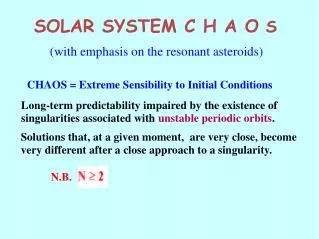
SOLAR SYSTEM C H A O S (with emphasis on the resonant asteroids) CHAOS = Extreme Sensibility to Initial Conditions Long-term predictability impaired by the existence of singularities associated with unstable periodic orbits. Solutions that, at a given moment, are very close, become very different after a close approach to a singularity. N.B.
-- Thule -- gap 2:1 -- Hildas -- Trojans -- gap 3:1 -- gap 7:3 -- gap 5:2 Distribution of the Asteroids with diameters larger than 90 km
Main tools for diagnostic of chaos Surfaces of Section (for N=2) Lyapunov Characteristic Exponents Fourier Analysis Spectral Number Frequency Map Analysis
Surface of Section of a System with regular orbits To Jupiter's Perihelion Polar coordinates: Radius Vector = Orbital Eccentricity Polar Angle = Position of Perihelion (Asteroid-Jupiter)
Surface of Section of an Integrable System Saddle-point (Unstable periodic orbit)
The homoclinic tangle cf. Contopoulos & Polymilis [Phys. Rev. E, 47, 1546 (1993)]
3-body planar model: Sun-Jupiter-asteroid with Jupiter in an Elliptic orbit and averaging over short-period angles. (at Low eccentricity) POLAR COORDINATES Radius Vector Orbital Eccentricity Polar Angle Position of Perihelion (Asteroid–Jupiter) To Jupiter's Perihelion
J.Wisdom, Astron. Journal 85 (1982) 0.4 0.3 0.2 0.1 0 Eccentricity 0 50 100 150 200 TEMPO (kyr)
Asteroids distribution in the neighborhood of the 3/1 resonance --Mars crossing line
0.6 Poincaré Map showing the low and medium-eccentricity modes of motion and their confinement by regular tori. To Jupiter's Perihelion Polar coordinates: Radius Vector = Orbital Eccentricity Polar Angle = Position of Perihelion (Asteroid-Jupiter)
(Very-high-eccentricity model) SFM & Klafke, NATO-ASI Proc. (1991) Phase portrait of the 3:1 Asteroidal Resonance To Jupiter's Perihelion New mode of motion around the stable corotation (e ~ 0.7) Polar coordinates: Radius Vector = Orbital Eccentricity (e<0.95) Polar Angle = Position of Perihelion (Asteroid-Jupiter)
(Very-high-eccentricity model) SFM & Klafke, NATO-ASI Proc. (1991) Eccentricity Jumps
SFM & Klafke, NATO-ASI Proc. (1991) Phase portrait of the 3:1 Asteroidal Resonance showing the rising of a homoclinic bridge To Jupiter's Perihelion the bridge Polar coordinates: Radius Vector = Orbital Eccentricity (e<0.95) Polar Angle = Position of Perihelion (Asteroid-Jupiter)
Half-life ~ 2.4 Myr --- (Gladman et al. 1997) Asteroids in the neighborhood of the3:1 resonance -- Venus Crossing Line -- Earth Crossing Line
Asteroid (4179) TOUTATIS (1.9 x 2.4 x 4.6 km) Radar image: Aug 12, 1992 (at 3.6 million km from Earth) Next close approach: Sep. 29, 2004 (1.55 million km from Earth) Rotation around the largest axis: 5.41 days Precession of the largest axis: 7.35 days
Methodology: Numerical simulations of the exact equations with Everhart's RA15 Integrator and Michtchenko's on-line low-pass filter. Would the model that succesfully explained the 3/1 resonance gap be able to explain the Hecuba gap? And the Hilda group? Answer: NO ! Ref: SFM, Astron. J. 108 (1994)
-- Thule -- gap 2:1 -- Hildas -- Trojans -- gap 3:1 -- gap 7:3 -- gap 5:2 Distribution of the Asteroids with diameters larger than 90 km
Surfaces of Section of the 2:1 asteroidal resonance. Model Sun-Jupiter-asteroid (planar)
Surfaces of Section of the 3:2 asteroidal resonance. Model Sun-Jupiter-asteroid (planar) Note: The scale was doubled. The regular regions are much smaller than before.
New improved model : 4 interacting bodies: Sun – Jupiter – Saturn – asteroid 3-D (but low inclination) The averaged model has more than 2 degrees of freedom. 2-D Surfaces of section no longer possible. The use of other diagnostic tools becomes necessary
Oseledec, Trudy Mosk. Mat. Ob. 1968 Benettin et al., Physical Review, 1976. LYAPUNOV CHARACTERISTIC EXPONENTS A measurement of the divergence of the bundle of neighboring solutions. where
Ref: SFM, IAU Symp. 160 (1994) LYAPUNOV TIMES = 1/max LCE Estimated from numerical integrations over 5-7 Myr in the range 0.1 < e < 0.4 and i=5 deg. 2:1 RESONANCE LYAPUNOV TIMES= 3000 yr to 0.3 Myr 3:1 RESONANCE LYAPUNOV TIMES = 0.3 to 10 Myr
(*) Interpretation of the results with the LECAR-FRANKLIN RULE 1.8 0.1 Sudden Orbital Lyap Transitions The rule: T ~ T (years) Sudden Trans. ~ Sudden Trans. ~ 2:1 Resonance: T > 10 Myr 3:2 Resonance T > 10 Gyr The dynamics of te 2:1 and 3:2 resonance are very similar, but the times for chaotic diffusion in the 3:2 resonance are larger than the age of the Solar System. (*) F.Franklin & M.Lecar, 1994 (Icarus).
FOURIER ANALYSIS – REGULAR SYSTEMS The solutions of a regular system are, in general, quasi- periodic. The Fourier analyisis of one solution shows as many peaks as the number of degrees of freedom of the system together with their main beats and harmonics. Log scale used to enhance small peaks.
FREQUENCY MAP ANALYSIS (J. Laskar) The frequency of a chosen peak in the spectra of the solution in two subsequent time intervals are compared. The variation of the frequency is a measurement of the chaotic behaviour of the solution. (This variation, in the case of a regular system, is zero).
Dynamical Map of 2/1 resonance. The Hecuba gap Refs: Nesvorny & SFM Icarus 130 (1997) SFM, Cel. Mech. Dyn. Astron. 73 (1999)
Dynamical Map of 3/2 resonance and the Hildas White dots: Actual asteroids ~30 with >50 km Refs: Nesvorny & SFM Icarus 130 (1997) SFM, Celest. Mech. Dyn. Astron. 73 (1999)
Chaos in Planetary Systems Some max LCEs Inner planets 5 Myr (Laskar, 1989) Pluto 20 Myr (Sussman & Wisdom, 1988)
FOURIER ANALYSIS – CHAOTIC SYSTEMS The solutions of a chaotic system are not quasi-periodic. The Fourier analyisis of one solution shows many apparently unrelated significant frequencies. Ref: Powell & Percival, J.Phys. A, 12, 2053 (1979)
SPECTRAL NUMBER (T.A.Michtchenko) The complexity of the spectrum is characterized by reckoning the number of peaks higher than a given level (5% of the highest peak in the examples shown) in the FFT of a suitable sampling of the solution.
And F8 V L=3L_sun d=13.47 pc M=1.3 M_sun age 2-3 Gyrs Absence of astrometric variation means sin i > 0,4 (i > 25deg) Absence of transits means sin i < 0.9925 (i < 83 deg)
Dynamical map of the Neighborhoof of planet And D (if i=30 deg) cf. Robutel & Laskar (2000) unpublished white spot: actual position of ups-And D Colision line with planet C chaotic regular
Neighbourhood of the 3rd planet of pulsar 1257 +12 3/2 Grid 21x51
A larger neighbourhood Grid: 21x101