Download
1 / 49
490 likes | 602 Vues
Tutorial „Modelling in the language XL“ University of Göttingen (Germany), September 21/22, 2009 Winfried Kurth Some basic examples in XL (part 2) related material: XL code files sm09_e??.rgg URL http://www.uni-forst.gwdg.de/~wkurth/ and drive T:gg on CIP pool stations.

E N D
Tutorial „Modelling in the language XL“ University of Göttingen (Germany), September 21/22, 2009 Winfried Kurth Some basic examples in XL (part 2) related material: XL code files sm09_e??.rgg URL http://www.uni-forst.gwdg.de/~wkurth/ and drive T:\rgg on CIP pool stations
interpretive rules insertion of a further phase of rule application directly preceding graphical interpretation (without effect on the next generation) application of interpretive rules interpretation by turtle
Example: module MainBud(int x) extends Sphere(3) {{setShader(GREEN);}}; module LBud extends Sphere(2) {{setShader(RED);}}; module LMeris; module AMeris; module Flower; const float d = 30; const float crit_dist = 21; protected void init() [ Axiom ==> MainBud(10); ] public void run() { [ MainBud(x) ==> F(20, 2, 15) if (x > 0) ( RH(180) [ LMeris ] MainBud(x-1) ) else ( AMeris ); LMeris ==> RU(random(50, 70)) F(random(15, 18), 2, 14) LBud; LBud ==> RL(90) [ Flower ]; AMeris ==> Scale(1.5) RL(90) Flower; /* Flower: here only a symbol */ ] applyInterpretation(); /* call of the execution of interpretive rules (to be done in the imperative part { ... } !) */ } protected void interpret() /* block with interpretive rules */ [ Flower ==> RH(30) for ((1:5)) ( RH(72) [ RL(80) F(8, 1, 9) ] ); ]
further example: public void run() { [ Axiom ==> A; A ==> Scale(0.3333) for (int i:(-1:1)) for (int j:(-1:1)) if ((i+1)*(j+1) != 1) ( [ Translate(i, j, 0) A ] ); ] applyInterpretation(); } public void interpret() [ A ==> Box; ] generates the so-called „Menger sponge“ (a fractal)
public void run() {[ Axiom ==> A; A ==> Scale(0.3333) for (int i:(-1:1)) for (int j:(-1:1)) if ((i+1)*(j+1) != 1) ( [ Translate(i, j, 0) A ] ); ] applyInterpretation(); } public void interpret() [ A ==> Box; ] (a) (b) (c) A ==> Box(0.1, 0.5, 0.1) Translate(0.1, 0.25, 0) Sphere(0.2); A ==> Sphere(0.5);
what is generated by this example? public void run() { [ Axiom ==> [ A(0, 0.5) D(0.7) F(60) ] A(0, 6) F(100); A(t, speed) ==> A(t+1, speed); ] applyInterpretation(); } public void interpret() [ A(t, speed) ==> RU(speed*t); ]
The step towards graph grammars drawback of L-systems: • in L-systems with branches (by turtle commands) only 2 possible relations between objects: "direct successor" and "branch" extensions: • to permit additional types of relations • to permit cycles graph grammar
a string: a very simple graph • a string can be interpreted as a 1-dimensional graph with only one type of edges • successor edges (successor relation) A A B C A A B C A
to make graphs dynamic, i.e., to let them change over time: graph grammars example rule:
A relational growth grammar (RGG) (special type of Graph grammar) contains: • an alphabet • the definition of all allowed • node types • edge types (types of relations) • the Axiom • an initial graph, composed of elements of the alphabet • a set of graph replacement rules.
How an RGG rule is applied • each left-hand side of a rule describes a subgraph (a pattern of nodes and edges, which is looked for in the whole graph), which is replaced when the rule is applied. • each right-hand side of a rule defines a new subgraph which is inserted as substitute for the removed subgraph.
a complete RGG rule can have 5 parts: (* context *), left-hand side, ( condition ) ==> right-hand side { imperative XL code }
in text form we write (user-defined) edges as -edgetype-> edges of the special type "successor" are usually written as a blank (instead of -successor->) also possible: >
2 types of rules for graph replacement in XL: ● L-system rule, symbol: ==> provides an embedding of the right-hand side into the graph (i.e., incoming and outgoing edges are maintained) ●SPO rule, symbol: ==>> incoming and outgoing edges are deleted (if their maintenance is not explicitely prescribed in the rule) „SPO“ from „single pushout“ – a notion from universal algebra
example: a:A ==>> a:A C (SPO rule) B ==> D E (L-system rules) C ==> A start graph: A B C
a:A ==>> a:A C (SPO rule) B ==> D E (L-system rules) C ==> A A B C D E A
a:A ==>> a:A C (SPO rule) B ==> D E (L-system rules) C ==> A A B C a: D E A
a:A ==>> a:A C (SPO rule) B ==> D E (L-system rules) C ==> A A D E A a: = final result C
test the example sm09_e27.rgg : module A extends Sphere(3); protected void init() [ Axiom ==> F(20, 4) A; ] public void runL() [ A ==> RU(20) F(20, 4) A; ] public void runSPO() [ A ==>> ^ RU(20) F(20, 4, 5) A; ] (^ denotes the root node in the current graph)
Mathematical background: see Chapter 4 of Ole Kniemeyer‘s doctoral dissertation (http://nbn-resolving.de/urn/resolver.pl?urn=urn:nbn:de:kobv:co1-opus-5937).
The language XL specification: Kniemeyer (2008) extension of Java allows also specification of L-systems and RGGs (graph grammars) in an intuitive rule notation procedural blocks, like in Java: { ... } rule-oriented blocks (RGG blocks): [ ... ]
Features of the language XL: ● nodes of the graph are Java objects (including geometry objects) example: XL programme for the Koch curve (see part 1) public void derivation() [ Axiom ==> RU(90) F(10); F(x) ==> F(x/3) RU(-60) F(x/3) RU(120) F(x/3) RU(-60) F(x/3); ] nodes of the graph edges (type „successor“)
special nodes: geometry objects Box, Sphere, Cylinder, Cone, Frustum, Parallelogram... access to attributes by parameter list: Box(x, y, z) (length, width, height) or with special functions: Box(...).(setColor(0x007700)) (colour)
special nodes: geometry objects Box, Sphere, Cylinder, Cone, Frustum, Parallelogram... transformation nodes Translate(x, y, z), Scale(cx, cy, cz), Scale(c), Rotate(a, b, c), RU(a), RL(a), RH(a), RV(c), RG, ... light sources PointLight, DirectionalLight, SpotLight, AmbientLight
Features of the language XL: ● rules organized in blocks [...], control of application by control structures example: rules for the stochastic tree Axiom ==> L(100) D(5) A; A ==> F0 LMul(0.7) DMul(0.7) if (probability(0.5)) ( [ RU(50) A ] [ RU(-10) A ] ) else ( [ RU(-50) A ] [ RU(10) A ] );
Features of the language XL: ● parallel application of the rules (can be modified: sequential mode can be switched on, see below)
Features of the language XL: ● parallel execution of assignments possible special assignment operator := besides the normal = quasi-parallel assignment to the variables x and y: x := f(x, y); y := g(x, y);
Features of the language XL: ● operator overloading (e.g., „+“ for vectors as for numbers)
Features of the language XL: ● set-valued expressions (more precisely: producer instead of sets) ● graph queries to analyze the actual structure
example for a graph query: binary tree, growth shall start only if there is enough distance to other F objects Axiom ==> F(100) [ RU(-30) A(70) ] RU(30) A(100); a:A(s) ==> if ( forall(distance(a, (* F *))> 60) ) ( RH(180) F(s) [ RU(-30) A(70) ] RU(30) A(100) ) without the „if“ condition with the „if“ condition
query syntax: a query is enclosed by (* *) The elements are given in their expected order, e.g.: (* A A B *) searches for a subgraph which consists of a sequence of nodes of the types A A B, connected by successor edges. test the examples sm09_e28.rgg, sm09_e29.rgg, sm09_e30.rgg, sm09_e31.rgg, sm09_e35.rgg, sm09_e36.rgg
Features of the language XL: ● aggregating operators (e.g., „sum“, „mean“, „empty“, „forall“, „selectWhereMin“) can be applied to set-valued results of a query
Queries and aggregating operators provide possibilities to connect structure and function example: search for all leaves which are successors of node c and sum up their surface areas query result can be transferred to an imperative calculation transitive closure aggregation operator
Queries in XL test the examples sm09_e28.rgg, sm09_e29.rgg, sm09_e30.rgg, sm09_e31.rgg, sm09_e35.rgg, sm09_e36.rgg
Representation of graphs in XL ● node types must be declared with „module“ ● nodes can be all Java objects. In user-made module declarations, methods (functions) and additional variables can be introduced, like in Java ● notation for nodes in a graph: Node_type, optionally preceded by: label: Examples: A, Meristem(t), b:Bud ● notation for edges in a graph: -edgetype->, <-edgetype- ● special edge types: successor edge: -successor->, > or (blank) branch edge: -branch->, +> or [ refinement edge: />
Notations for special edge types > successor edge forward < successor edge backward --- successor edge forward or backward +> branch edge forward <+ branch edge backward -+- branch edge forward or backward /> refinement edge forward </ refinement edge backward --> arbitrary edge forward <-- arbitrary edge backward -- arbitrary edge forward or backward (cf. Kniemeyer 2008, p. 150 and 403)
user-defined edge types const int xxx = EDGE_0; // oder EDGE_1, ..., EDGE_14 ... usage in the graph: -xxx->, <-xxx-, -xxx- Notation of graphs in XL example: is represented in programme code as (the representation is not unique!) ( >: successor edge, +: branch edge)
derived relations relation between nodes connected by several edges (one after the other) of the same type: „transitive hull“ of the original relation (edge)
Notation for the transitive hull in XL: (-edgetype->)+ reflexive-transitive hull („node stands in relation to itself“ also permitted): (-edgetype->)* e.g., for the successor relation: (>)* common transitive hull of the special relations „successor“ and „branch“, in reverse direction: -ancestor-> interpretation: this relation is valid to all „preceding nodes“ in a tree along the path to the root. nearest successors of a certain node type: -minDescendants->(nodes of other types are skipped)
successor edge branch edge minDescendants relation „ancestor“
The current graph • GroIMP maintains always a graph which contains the complete current structural information. This graph is transformed by application of the rules. • Attention: Not all nodes are visible objects in the 3-D view of the structure! • F0, F(x), Box, Sphere: yes • RU(30), A, B: normally not (if not derived by „extends“ • from visible objects) • The graph can be completely visualized in the 2-D graph view (in GroIMP: Panels - 2D - Graph).
Load an example RGG file in GroIMP and execute some steps (do not work with a too complex structure). Open the 2-D graph view, fix the window with the mouse in the GroIMP user interface and test different layouts (Layout - Edit): Tree Sugiyama Square Circle Random SimpleEdgeBased Fruchterman Keep track of the changes of the graph when you apply the rules (click on „redraw“)!
which parts of the current graph of GroIMP are visible (in the 3-D view) ? all geometry nodes which can be accessed from the root (denoted ^) of the graph by exactly one path, which consists only of "successor" and "branch" edges How to enforce that an object is visible in any case: ==>> ^ Object
Derivation modes in XL default: parallel application of rules (like in L-systems) to switch into sequential mode (then, in each step at most one rule is applied at one match): setDerivationMode(SEQUENTIAL_MODE) to switch back to parallel mode: setDerivationMode(PARALLEL_MODE) test the example sm09_e32.rgg
a further type of rules: actualization rules often, nothing at the graph structure has to be changed, but only attributes of one single node are to be modified (e.g., calculation of photosynthesis in one leaf). For this purpose, there is an extra rule type: A ::> { imperative code }; Test the examples sm09_e25.rgg, sm09_e16.rgg, sm09_e17.gsz, sm09_e18.rgg and concerning the access to node attributes: sm09_e26.rgg
Modelling diameter growth in plants • frequently used approaches: • regression diameter ~ length for new growth units • then, diameter increment dependent from age, branch order, • etc. • e.g., use rule with fixed annual growth • Shoot(l, d) ==> Shoot(l, d+delta_d); • interpretive rule for Shoot: Shoot(d) ==> F(l, d); • or: “pipe model“ assumption
“pipe model“ (SHINOZAKI et al. 1964) : parallel “unit pipes“ cross section area ~ leaf mass ~ fine root mass
conclusion: „Leonardo rule“ (da Vinci, about 1500) di In each branching node we have d2 = di2 (invariance of cross section area) d
A1 A = A1 + A2 d 2 = d12 + d22 A A2 realization in an XL-based model: see examples sm09_e33.rgg, sm09_e34.rgg there, first the structural and length growth is simulated, then in separate steps the diameter growth, calculated top-down (also a – more realistic – combination is possible)