Download
1 / 38
390 likes | 556 Vues
Chapter 2. Optimal Trees and Paths. Combinatorial Optimization 2012. 1. 2.1 Minimum Spanning Trees. Definitions about Graphs: graph , : set of nodes, : set of edges, relation associating with each edge a pair of its end nodes. simple graph : graph with no parallel edges, no loops

E N D
Chapter 2. Optimal Trees and Paths Combinatorial Optimization 2012 1
2.1 Minimum Spanning Trees • Definitions about Graphs: graph, : set of nodes, : set of edges, relation associating with each edge a pair of its end nodes. simple graph : graph with no parallel edges, no loops complete graph : simple graph such that every pair of nodes is the set of ends of some edge. subgraph of : , , and each has the same ends in as in . , : subgraphs.t., . , : delete and all edges incident with nodes in . is the subgraph induced by . spanning subgraph : Usually use , .
path from to , path : sequence such that the ends of are . (walk) closed path : path with . edge-simple path : distinct. (trail) simple path : . (path) circuit : edge-simple and closed path, distinct. (cycle) length of path : number of edge-terms of . • is connected if every pair of nodes is joined by a path. • is cut node of connected graph if is not connected. • Similar definitions for directed network.
b h 31 28 32 d 16 18 15 22 23 a g 29 12 k 35 20 25 f • Connector Problem Given a connected graph and a positive cost for each , find a minimum cost spanning connected subgraph of .
Lemma 2.1: An edge of is an edge of a circuit of if and only if there is a path in from to . • We still have a connected graph if we delete an edge of some circuit. So an optimal solution to the connector problem will not have any circuits since edge costs are positive. • Def: forest: a graph having no circuit ( acyclic graph ) tree: connected forest ( connected acyclic graph ) • Minimum spanning tree problem Given a connected graph and a real cost for each , find a minimum cost spanning tree of .
Prop: Following conditions are equivalent in defining a tree. • is a forest containing edges. • Edge-minimal connected graph spanning . • Contains a unique path between each pair of nodes of . • The addition of any one edge not in creates a unique cycle. • Greedy style MST algorithms: • Kruskal’s algorithm • Prim’s algorithm
Kruskal’s algorithm for MST Keep a spanning forest of with initially. At each step add to a least-cost edge such that remains a forest. (sort the edges and use them sequentially) Stop when is a spanning tree. b h 31 28 32 d 16 18 15 22 23 a g 29 12 k 35 20 25 f
Prim’s algorithm for MST Keep a tree with initially for some , and initially. At each step add to a least-cost edge e not in such that remains a tree. Stop when is a spanning tree. 31 b h 28 32 d 16 18 15 22 23 a g 29 12 k 35 20 25 f
Validity of MST algorithms • Notation: Let . = { : has an end in and an end in } = { : both ends of are in } (also denoted as freq.) for some is called a cut of (similar definition for directed graph, for some . -cut is a cut for which .) • Thm 2.3: is connected if and only if there is no set , with . Pf) Show contraposition in both directions. ) If for some nontrivial and , , there is no path from to , hence is not connected. ) If is not connected, there exists such set .
Def: is called extendible to an MST if is contained in the edge-set of some MST of . • Thm 2.4: Suppose and is extendible to an MST. Edge is a minimum cost edge of some cut with . Then is extendible to an MST. • Lemma 2.7: Let be a spanning tree of . Let be an edge of but not , and let be an edge of a simple path in from to . Then the subgraph is a spanning tree of . • Pf of Them 2.4) Let be an MST such that . If , then done. Suppose . Let be a simple path in from to () such that . Then , hence is also an MST by Lemma 2.7. From is extendible to an MST.
See text Thm 2.5, Thm 2.6 for correctness of the Kruskal and Prim’s algorithms. • Also see the text for running time of the algorithms. • Prim’s alg.: • Kruskal’s alg.: (sorting m edges)
MST and LP • Notation: set , vector and any , let . • IP formulation of MST problem min (2.1) , for all , (2.2) (2.3) , for all ( and integer, for all ) (2.4) ( edges and no cycles, subtour elimination formulation. )
Linear programming relaxation: drop integrality requirements = min (2.1) , for all (2.2) (2.3) for all (2.4) • { feasible solutions to IP} { feasible solutions to LP relaxation} Hence , i.e. provides a lower bound on optimal IP value. Upper bound on usually obtained by finding a feasible solution to IP. If lower bound = upper bound, then we have found optimal value. • For MST problem, .
We know that there exists an extreme point optimal solution of a linear programming problem if the LP has finite optimal value. (With the assumption that the underlying polyhedron has an extreme point.) So, if all extreme points of the feasible solution set of LP are integer vectors, we can find integer optimal solution by solving the LP relaxation. • Results to be proved later: If the LP relaxation has an integer optimal solution for any cost vector , all the extreme points of the feasible solution set of the LP are integer vectors. • Suppose we have two types of correct formulations for the same problem (in minimization form). Consider the LP relaxations and corresponding polyhedra and with . Then , hence LP relaxation over provides more tight lower bound, which can be quite helpful in solving the IP problem by branch-and-bound.
Idea of Branch-and-Bound Algorithm • Solution set is non-convex. Difficult to solve. • Idea : divide and conquer. Divide feasible solutions set into many disjoint sets. Find the best solution for each subset. Then choose the best one. To divide the feasible solutions set, we add linear inequalities to the problem. (e.g. , , … ) But the divided problem is still integer programming problem. So we need a means to find the best integer solution for each integer programming problem. • Linear programming relaxation : (IP) (LPR)
Let be the optimal value of (IP) and be the optimal value of (LPR) If is a feasible solution to (IP) feasible solution to (LPR) Hence {set of feasible solutions to (IP) } { set of feasible solutions to (LPR) } and objective function is the same. Also a feasible solution to (IP) provides an upper bound on . Hence if we solve (LPR) and obtain optimal solution which happens to be integral, then the solution provides an upper bound which is the same as the lower bound. It implies that the solution is optimal to the integer programming problem. If the obtained solution is not integral, we only have lower bound on optimal value. Then we divide the feasible solution set and repeat the procedure again for each divided problem. • Note that other schemes are possible to obtain lower bound on , other than the linear programming relaxation. (e.g., Lagrangian relaxation, dual problems, …)
Results of solving LP relaxation. • unbounded integer program unbounded • infeasible integer program infeasible • optimal solution which is integer it is optimal to integer program • optimal solution not integer only obtain lower bound. Need to branch • How to divide the solution set in case of 4. Suppose x* optimal solution to LP relaxation and Then consider 2 sets Any feasible solution to integer program is contained in one of (a), (b). So we do not miss any feasible solution. Then we solve LP relaxation of (a), (b) again. (Search procedure with tree structure)
Useful tool to facilitate the search: Suppose x* is the best solution currently known and its objective value is z*. If the LP relaxation of a subproblem gives optimal value such that we know that there does not exist an integer solution in this subproblem which gives objective value smaller than z*. Hence we do not need to explore the subproblem any further and prune the subproblem (the corresponding node in the branch-and-bound tree). • Obtaining a good (large) lower bound in each subproblem is important to reduce the number of subproblems examined. Modern approach adds more valid inequalities to tighten the feasible region (cutting plane approach).
Procedure to solve the LP relaxation (with many constraints) Cutting plane approach Solve LP relaxation with small number of constraints (e.g., w/o subtourelim. constr.) If satisfies all constr., stop. O/w find a violated constr. (separation problem) Solve LP after adding the violated constraint. Y violated constr? N Stop
Alternative formulation for MST and LP relaxation min (2.1*) , for all (2.2*) (2.3*) and integer, for all (2.4*) ( edges and connected, cutset formulation. ) • The polyhedron of the LP relaxation of subtour elimination formulation is properly contained in the polyhedron for cutset formulation. Hence LP relaxation of the subtourelim. formulation provides stronger bound. ( see handout ) Moreover, the extreme points of the polyhedron for the LP relaxation of the subtourelim. formulation are integer vectors.
General questions for a problem: Extreme points of LP relaxation all integer vectors? If not, can we make the polyhedron have only integer extreme points by adding some inequalities to the LP relaxation? How much efforts? If not, can we approximate the integer polyhedron using only part of the inequalities needed to describe it? (obtain good lower bound) How much efforts?
Thm 2.8: Let be the characteristic vector of an MST with respect to costs . Then is an optimal solution of (2.1). Pf) Consider a form equivalent to (2.1). Let , number of components in subgraphof . = min (2.1) , for all (2.2) (P1) (2.3) , for all (2.4) = min (2.5) , for all (2.6) (P2) (2.7) , for all (2.8) Let be the node sets of the components in Interpret as .
Let be the characteristic vector of an MST. Then is a feasible solution of . Hence provides a lower bound on the cost of an MST. • Problem has the same feasible solutions as . We will consider to prove Thm 2.8.
( Given , we say that is independent if there is no cycle in . (2.6) means that the cardinality of a maximal independent set in should not exceed . More in Chap. 8 Matroids. ) (2.6) (2.2) (i.e. ) Let . Then since . (2.2) (2.6) (i.e. ) Take nonnegative linear combination of (2.2) and . Let be node sets of the components in Add lhs and rhs of (2.2) respectively for . . Add for the edges in but not in to eliminate them from lhs.
Let be the characteristic vector generated by Kruskal’s algorithm. (We do not need to assume that it is optimal by now) We show that is optimal to (2.5) by providing a dual feasible solution satisfying complementary slackness conditions with . Consider the form max , then dual is min (2.9) s.t., for all (2.10) , for all , free (2.11) Let be the sorted sequence in Kruskal’s algorithm . Let . Construct dual solution as follows. , if is not one of , ( ) , Hence , .
Check dual feasibility of . For ( th edge considered in K’s alg.), dual feasible and part of CS conditions satisfied ( corresponding dual constraint at equality ) Need to show corresponding primal constr. active at . We know for some has . Consider a with and suppose (2.6) does not hold at equality for this . Then some edge in whose addition to decreases the number of components in . Such edge would have been added to by K’s algorithm. Proof here also shows alternatively that K’s algorithm gives an optimal solution since we did not assume that the solution obtained by K’s algorithm is optimal in the proof.
Thm 2.8 can be used to examine the strength of the bound obtained by 1-tree relaxation (Lagrangian relaxation) for traveling salesman problem. • Why consider IP (LP) formulation for MST although efficient algorithms for it? • Other variations of MST: • degree constrained spanning tree: degree of each node should be k for all v V. (NP-hard) • shortest total path length spanning tree: sum of path lengths between every pair u, v is minimum. (NP-hard) • Steiner tree problem: Given , , costs . Find the min cost tree spanning . (NP-hard) ….
Steiner tree problem • Given , costs . Find the min cost tree spanning (called terminal nodes). • Formulation = min , for all , , for all integer
Consider directed version of the Steiner tree problem (Steiner arborescence problem) • We duplicate each edge by two antiparallel arcs with same costs , obtaining directed graph . Choose some , which we call the root. A Steiner arborescence (rooted at ) is a set of arcs such that is a directed subtree that contains a directed path from to for all . Note the one-to-one correspondence between a Steiner tree and its directed version (Steiner arborescence), hence can find an optimal Steiner arborescence and recover the optimal Steiner tree.
Example of a Steiner arborescence : Terminal nodes b h {r} a g k f
Formulation for Steiner arborescence problem = min , for all , , , , for all integer , where • Any in the formulation is a cut for some . Suppose we solve the LP relaxation by cutting plane algorithm. Given a current solution , we assign as arc capacities, and find minimum cut for all for separation. • It can be shown that the LP relaxation of the directed version gives stronger lower bound than the undirected version although it has twice as many variables. Computationally successful. • There are other formulations and algorithms (e.g., dynamic programming) for Steiner tree problems, too.
Models for Connectivity of Graphs • Motivation: Design network that can survive link and/or node failure. MST is the cheapest network structure that provides connectivity, but failure of an edge or node results in disruption of communication. We want to achieve the survivability of network in case of failure at minimum cost. • Problem: Given undirected , costs , find subgraph, that satisfies certain connectivity requirements at minimum cost.
Definitions in terms of paths (See handouts) • Def: Two nodes are called edge (vertex or k-) connected if there exist edge-disjoint (internally disjoint, vertex-disjoint) simple paths between and . • Def: A graph is called edge (vertex or k-) connected if all pairs of distinct nodes of are edge (vertex) connected. • Def: For graph , the largest integer such that is edge connected (vertex connected) is called the edge connectivity (vertex connectivity, or connectivity) of and denoted .
Connectivity also can be defined in terms of edge cut and node (vertex) cut. • Def:edge cut is an edge cut ( for some ) of elements. (Edge connectivity ( ) of is minimum for which has a edge cut. is called edge connected if .) • Def:Let and be distinct nonadjacent vertices of . An -vertex cut is a subset of such that and belong to different components of . A vertex cut separating some pair of nonadjacent vertices of is a vertex cut of , and one with elements is a -vertex cut. (Node connectivity () of is minimum for which has a vertex cut. is called vertex (or connected if ._
Menger’sThm states that both definitions for edge-connectivity (node-connectivity) are equivalent. • Thm9.1(Menger’sThm, handout): In any graph , where and are nonadjacent, the maximum number of pairwise internally disjoint paths is equal to the minimum number of vertices in an vertex cut. (). Pf) May consider later after studying max flow min cut Theorem. Refer Bondy and Murty Chap 3 and p.203 – 205 (1976), and handout. • Thm 9.2: If has at least one pair of nonadjacent vertices, min . Pf) See handout. • Similar results hold for edge-connectivity. Also for directed graph.
IP models for connectivity: see handout Survivability requirements : there must exist edge disjoint paths in : removal of at most nodes (except ) must leave at least edge disjoint paths. • Formulation: min s.t (i) , and such that (ii) , and with and with (iii) , (iv) integral,
Special cases: • MST: drop (ii), set , (assuming ) • Steiner tree problem: drop (ii), set , otherwise • Min cost edge connected network: drop (ii) • Min cost k-node connected network: drop (i) • Practical models: define node type for , min satisfies node survivability (edge survivability) conditions if for all , there exist node disjoint (edge disjoint) paths. ( conduit level network design) • There can be different IP formulations for the respective problems.
The structure of the survivable network may depend on the facilities used (e.g. ADM (Add-Drop Multiplexor) needs to configure ring networks )