Principles of Parallel Algorithm Design
This chapter discusses the principles of parallel algorithm design, including task decomposition, processes and mapping, and processes versus processors. It also explores preliminaries such as decomposition, tasks, and dependency graphs.


Principles of Parallel Algorithm Design
E N D
Presentation Transcript
Principles of Parallel Algorithm Design To accompany the text “Introduction to Parallel Computing”, Addison Wesley, 2003. Ananth Grama, Anshul Gupta, George Karypis, and Vipin Kumar
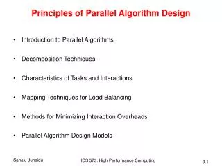
Chapter Overview: Algorithms and Concurrency • Introduction to Parallel Algorithms • Tasks and Decomposition • Processes and Mapping • Processes Versus Processors
Preliminaries: Decomposition, Tasks, and Dependency Graphs • The first step in developing a parallel algorithm is to decompose the problem into tasks that can be executed concurrently • A given problem may be decomposed into tasks in many different ways. • Tasks may be of same or different sizes. • A decomposition can be illustrated in the form of a directed graph with nodes corresponding to tasks and edges indicating that the result of one task is required for processing the next. Such a graph is called a task dependency graph.
Example: Multiplying a Dense Matrix with a Vector Computation of each element of output vector y is independent of other elements. Based on this, a dense matrix-vector product can be decomposed into n tasks. The figure highlights the portion of the matrix and vector accessed by Task 1. Observations: While tasks share data (namely, the vector b ), they do not have any control dependencies - i.e., no task needs to wait for the (partial) completion of any other. All tasks are of the same size in terms of number of operations. Is this the maximum number of tasks we could decompose this problem into?
Example: Database Query Processing Consider the execution of the query: MODEL = ``CIVIC'' AND YEAR = 2001 AND (COLOR = ``GREEN'' OR COLOR = ``WHITE) on the following database:
Example: Database Query Processing The execution of the query can be divided into subtasks in various ways. Each task can be thought of as generating an intermediate table of entries that satisfy a particular clause. Decomposing the given query into a number of tasks. Edges in this graph denote that the output of one task is needed to accomplish the next.
Example: Database Query Processing Note that the same problem can be decomposed into subtasks in other ways as well. An alternate decomposition of the given problem into subtasks, along with their data dependencies. Different task decompositions may lead to significant differences with respect to their eventual parallel performance.
Granularity of Task Decomposition • The number of tasks into which a problem is decomposed determines its granularity. • Decomposition into a large number of tasks results in fine-grained decomposition and that into a small number of tasks results in a coarse grained decomposition. A coarse grained counterpart to the dense matrix-vector product example. Each task in this example corresponds to the computation of three elements of the result vector.
Degree of Concurrency • The number of tasks that can be executed in parallel is the degree of concurrencyof a decomposition. • Since the number of tasks that can be executed in parallel may change over program execution, the maximum degree of concurrency is the maximum number of such tasks at any point during execution. • The average degree of concurrencyis the average number of tasks that can be processed in parallel over the execution of the program. • The degree of concurrency increases as the decomposition becomes finer in granularity and vice versa.
Critical Path • A directed path in the task dependency graph represents a sequence of tasks that must be processed one after the other. • start node : Node with no incoming edges • finish node:Node with no outgoing edges • The longest directed path between any pair of start and finish nodes is known as the critical path.Such path determines the shortest time in which the program can be executed in parallel. • The length of the critical path is called the critical path length. • How to compute the path length? • Calculate sum of the weights of nodes along this path, where the weight of a node is the size or the amount of work associated with the corresponding task.
Critical Path Consider the task dependency graphs of the two database query decompositions: • What are the critical path lengths for the two task dependency graphs? • If each task takes 10 time units, what is the shortest parallel execution time for each decomposition? • How many processors are needed in each case to achieve this minimum parallel execution time? • What is the maximum degree of concurrency?
Critical Path Consider the task dependency graphs of the two database query decompositions: • What is the average degree of concurrency? • The ratio of the total amount of work to the critical-path length is the average degree of concurrency. • shorter critical path gives a higher degree of concurrency.
Limits on Parallel Performance • It would appear that the parallel time can be made arbitrarily small by making the decomposition finer in granularity. • There is an inherent bound on how fine the granularity of a computation can be. • For example, in the case of multiplying a dense matrix with a vector, there can be no more than (n2) concurrent tasks. • Concurrent tasks may also have to exchange data with other tasks. This results in communication overhead. The tradeoff between the granularity of a decomposition and associated overheads often determines performance bounds.
Task Interaction Graphs • Subtasks generally exchange data with others in a decomposition. For example, even in the trivial decomposition of the dense matrix-vector product, if the vector is not replicated across all tasks, they will have to communicate elements of the vector. • The graph of tasks (nodes) and their interactions/data exchange (edges) is referred to as a task interaction graph. • task interaction graphs represent data dependencies, • task dependency graphs represent control dependencies.
Task Interaction Graphs: An Example Consider the problem of multiplying a sparse matrix A with a vector b. The following observations can be made: • As before, the computation of each element of the result vector can be viewed as an independent task. • Unlike a dense matrix-vector product though, only non-zero elements of matrix A participate in the computation. • If, for memory optimality, we also partition b across tasks, then one can see that the task interaction graph of the computation is identical to the graph of the matrix A.
Task Interaction Graphs: An Example • Assign the computation of the element y[i] of the output vector to Task i, • make Task ithe "owner" of row A[i, *] of the matrix and the element b[i] of the input vector. • As a result, computation of y[i] requires access to many elements of b that are owned by other tasks. So Task imust get these elements from the appropriate locations. • Task ishould send b[i] to all the other tasks that need it for their computation. For example, Task 4 must send b[4] to Tasks 0, 5, 8, and 9 and must get b[0], b[5], b[8], and b[9] to perform its own computation.
Processes and Mapping • In general, the number of tasks in a decomposition exceeds the number of processing elements available. • For this reason, a parallel algorithm must also provide a mapping of tasks to processes. Note: We refer to the mapping as being from tasks to processes, as opposed to processors. This is because typical programming APIs do not allow easy binding of tasks to physical processors. Rather, we aggregate tasks into processes and rely on the system to map these processes to physical processors. We use processes, not in the UNIX sense of a process, rather, simply as a collection of tasks and associated data.
Processes and Mapping • Appropriate mapping of tasks to processes is critical to the parallel performance of an algorithm. • Mappings are determined by both the task dependency and task interaction graphs. • Task dependency graphs can be used to ensure that work is equally spread across all processes at any point (minimum idling and optimal load balance). • Task interaction graphs can be used to make sure that processes need minimum interaction with other processes (minimum communication).
Processes and Mapping An appropriate mapping must minimize parallel execution time by: • Mapping independent tasks to different processes. • Assigning tasks on critical path to processes as soon as they become available. • Minimizing interaction between processes by mapping tasks with dense interactions to the same process. • Note: These criteria often conflict with each other. For example, a decomposition into one task (or no decomposition at all) minimizes interaction but does not result in a speedup at all!
Processes and Mapping: Example • Mapping tasks in the database query decomposition to processes. • Amaximum of four processes can be used. This is because the maximum degree of concurrency is only four. • Map the tasks connected by edges to one task, onto the same process because this prevents an inter-task interaction from becoming an inter-processes interaction.