Data collection and analysis

1. Data collection and analysis Jørn Vatn NTNU

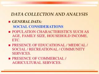
2. Objectives data collection and analysis • Collection and analysis of safety and reliability data is an important element of safety management and continuous improvement • There are several aspects of utilizing experience data and we will in the following focus on • Learning from experience • Identification of common problems • “Top ten”-lists (visualized by Pareto diagrams) • A basis for estimation of reliability parameters • MTTF, MDT, aging parameters

3. Collection of data • We differentiate between • Accident and incident reporting systems • These data is event-based, i.e. we report into the system only when critical events occur • Examples of such system is Synergy, and Tripod Delta • Databases with the aim of estimating reliability parameters • These databases contains system description, failure events, and maintenance activities • The Offshore Reliability Data (OREDA) is one such database • Such databases will be denoted RAMS databases in the following

4. A clear boundary description is imperative for collecting, merging and analyzing RAMS data from different industries, plants or sources The merging and analysis will otherwise be based on incompatible data. For each equipment class a boundary must be defined. The boundary defines what RAMS data are to be collected RAMS data: Boundary description

5. RAMS Data:Equipment hierarchy • The highest level is the equipment unit class • The number of levels for subdivision will depend on the complexity of the equipment unit and the use of the data

6. Data categories • Equipment data • Failure data • Maintenance data • State information

7. RAMS database structure

8. Equipment data • Identification data; e.g. • equipment location • classification • installation data • equipment unit data; • Design data; e.g. • manufacturer’s data • design characteristics; • Application data; e.g. • operation, environment

9. Equipment data (Adapted from ISO 14224)

10. Failure data • identification data, failure record and equipment location; • failure data for characterizing a failure, e.g. failure date, maintainable items failed, severity class, failure mode, failure cause, method of observation

11. Failure data (From ISO 14224)

12. Failure causes (Failure descriptors, From ISO 14224)

13. Failure causes, cont

14. Failure causes, cont

15. Failure causes, cont

16. Failure causes, cont

17. Maintenance data • Maintenance is carried out • To correct a failure (corrective maintenance); • As a planned and normally periodic action to prevent failure from occurring (preventive maintenance).

18. Maintenance data (From ISO 14224)

19. State information • State information (condition monitoring information) may be collected in the following manners: • Readings and measurements during maintenance • Observations during normal operation • Continuous measurements by use of sensor technology

20. State information, discrete readings

21. State information, continuous readings

22. Data analysis • Graphical techniques • Histogram • Bar charts • Pareto diagrams • Visualization of trends • Parametric models • Estimation of constant failure rate • Estimation of increasing hazard rate • Estimation of global trends (over the system lifecycle)

23. Pareto diagram (“Top ten”, components)

24. Presenting raw data and rates from accident and incident reporting systems • When presenting a “snapshot” of the indicators we often compare with targets value • Colour codes may be used • For “occurrences” we just plot the raw data • For frequencies we need to establish the “exposure” • Number of working hours in the period • Number of critical work operations

25. Cross-tabulation • To see the effect of explanatory variables we could plot the number of occurrence or frequencies as a function of one or two explanatory variables •  we get an indication whether the risk is unexpected high among certain groups of workers, during specific work operations, in special periods etc

26. Example of cross tabulation (dummy figures)

27. Root cause analysis • The objective is to present the contributing factors to the HSE indicators • Occurrences and/or frequencies are plotted against the causation codes, see next slide • Challenges • How to treat more than one causation code? • Causation codes are organised in a structure

28. Causation codes in an MTO structuring • Triggering factors • Underlying causes • Work organisation • Work supervision • Change routines • Communication • Working environment • Requirements/procedures/guidelines • Management of company/entity • Deficient safety culture • Poor quality of established systems

29. HSE deviations per triggering factor

30. Trend curves, three alternatives • Plot number of occurrences as a function of time (histogram) • Plot frequencies (number/exposure) as a function of time • Plot both number and exposure as a function of time in the same diagram

31. Quarterly HSE deviation Exposure (hours worked) Incidents

32. Challenges • Difficult to see trends due to the stochastic nature of the number of events • As an alternative, plot cumulative number of events as a function of time (adjusted for exposure) • Convex plot indicates increasing risk level • Concave plot indicates an improving situation • The following example is based on the previous plot

33. Cumulative number of deviations

34. Interpretation of cumulative plot • A convex plot indicates an increasing frequency of incidents () • A concave plot indicates improvement ()

35. Note • Cross-tabulation and trend curves are used to focus on safety problems, but do not indicate improvement measures • Root cause analysis identifies significant causes behind the undesired events/accidents  cue on measures • Risk reducing measure should be based on an understanding of • That the measure is directed against one or more failure causes (causation code) • That the measure is effective in terms of e.g., cost • That no negative effects of the measure is anticipated

36. Parameter estimation /bathtub curve • The bathtub curve is a basis for reliability modelling, but • There are two such curves • The hazard rate for ”local time” • The failure intensity for ”global time” • Combining the two:

37. Performance loss

38. Plotting techniques, lifetime data (local bath tubcurve) • Several plots exists to visualize characteristics of lifetime data • TTT-plot • Kaplan-Meier plot • Hazard plot • All these plots assume • Failure times are identical,and independent distributes • I.e. no change over system lifetime • Examples of how life timesare generated are shown to the right

39. TTT- Total Time on Test plot • Let T1,T2,T3,..,Tn be the recorded lifetimes • Let T(1),T(2),T(3),.. be ordered lifetimes, i.e. T(1)T(2)T(3).. • Define the total test on time at time t by • where i is such that T(i)t < T(i+1) • The TTT-plot is obtained by plotting for i = 1,..,n:

40. Example

41. Example plot

42. Interpretation • A plot around the diagonal indicates a constant hazard rate, i.e. failure times can be considered exponentially distributed. • A concave plot (above the diagonal) indicates an increasing hazard rate (IFR). • A convex plot (under the diagonal) indicates a decreasing hazard rate (DFR). • A plot which fist is convex, and then concave indicates a bathtub like hazard rate • A plot which first is concave, and then convex indicates heterogeneity in the data, see Vatn (1996).

43. Exercise • Assume that the following failure data for one component type has been recorded (in months) • 8,9,7,6,12,18,14,6,9,11,24 • Construct the TTT plot • What would you say about the hazard rate?

44. The Nelson Aalen plot for global trend over the system lifetime • The Nelson-Aalen plot shows the cumulative number of failures on the Y-axis, and the X-axis represents the time • A convex plot indicates a deteriorating system, whereas a concave plot indicates an improving system • The idea behind the Nelson-Aalen plot is to plot the cumulative number of failures against time • Actually we plot W(t) which is the expected cumulative numbers of failures in a time interval

45. Nelson Aalen procedure • When estimating W(t) we need failure data from one or more processes (systems) • Each process (system) is observed in a time interval (ai,bi] and tij denotes failure time j in process i (global or calendar time) • To construct Nelson Aalen plot the following algorithm could be used • Group all the tij’s and sort them, and denote the result tk, k = 1,2,….. • For each k, let Ok denote the number of processes that are under observation just before time tk • Let • Let, k = 1,2,… • Plot

46. Example of Nelson Aalen plot

47. Parameter estimation • Constant hazard rate, homogeneous sample • Constant hazard rate, non-homogeneous sample • Increasing hazard rate

48. Constant failure rate homogeneous sample • In this situation we only need the following information • t = aggregated time in service • n = the total number of observed failuresin the period • An estimate for the failure rate is given by

49. Multi-Sample Problems • In many cases we do not have a homogeneous sample of data • The aggregated data for an item may come from different installations with different operational and environmental conditions, or we may wish to present an “average” failure rate estimate for slightly different items • In these situations we may decide to merge several more or less homogeneous samples, into what we call a multi-sample • The various samples may have different failure rates, and different amounts of data

50. Illustration, multi-sample data