Simulation Techniques Overview
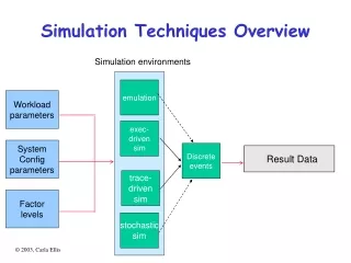
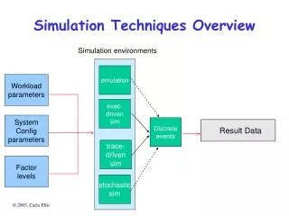
Simulation Techniques Overview. Simulation environments. emulation. Workload parameters. exec- driven sim. System Config parameters. Discrete events. Result Data. trace- driven sim. Factor levels. stochastic sim. The End Game: When to Stop. final conditions. transient interval.

Simulation Techniques Overview
E N D
Presentation Transcript
Simulation Techniques Overview Simulation environments emulation Workloadparameters exec-drivensim SystemConfigparameters Discreteevents Result Data trace-drivensim Factorlevels stochasticsim
The End Game: When to Stop finalconditions transientinterval steadystate b a t
Issues • If you stop at a – before the cleanup phase: • Must be careful in calculating metrics when some events are outstanding • Example: scheduling simulation. Some jobs completed and some still in queue. • Average service time must count just completed jobs. • Average queue length must be over time not queuing events. • If you stop at b – completion: • Not at steady state again • Example: jobs are finishing with no new arrivals
x ! z1-a/2Var(x) Var(x) = Var(x) n Stopping Criteria • Assuming you choose to stop at a – how to determine a? • Simulation should be run long enough for the confidence interval for the mean response to narrow to desired width • Variance of the sample mean of n independent observations uses variance of observations
Correlated Observations • Often the observations are not independent • Memory access time depends on cache state built by previous memory request • Waiting time depends on length of previous job • Solutions • Independent replications of simulation experiment • Batch means • Regeneration
Replications • m replications with different seed value each time, of size n+n0 where n0 is initial transient phase during which data is discarded. • Confidence interval is inversely proportional to mn • Increase either m or n to get narrower C.I. • Page 431 shows how to calculate overall mean for all replications, Var(x), and C.I.
Batch means • Subsamples – long simulation run of N + n0observations • Divide N observations into m samples of n observations each • Batch size n must be large enough so the batch means have little correlation • Compute covariance of successive batch means xi and xi+1 with bigger n’s until it is small enough n0 n n n t • C.I width again inversely proportional to mn
Regeneration • Independent phases where the execution returns to an initial state • Flushed cache • Empty job queue • Regeneration cycles may be of unequal length (complicates math – page 434) • m cycles of n1, n2, …, nm sizes s.t. C.I. is narrow enough Regenerationpoints t Regenerationcycle
Structure of Discrete Event Simulation scheduler eventQ State var Event handlers results
Role of Random Values in Discrete Event Simulation randomparameters scheduler e eventQ random values ininitializationof state State var Event handlers results
Random Values • Want random values with a specified distribution • Step 1: produce uniformly distributed numbers between 0 and 1(random number generation) • Step 2: apply transformation to produce values from desired distribution (random variate generation)
Random Number Generators xn = f ( xn-1, xn-2) where x0 is seed • Pseudo-random since, given the same seed, the sequence is repeatable and deterministic • Cycle length – length of repeating sequence • Example: xn = a xn-1 + b mod m seed cycle period
Desirable Properties • Period should be large • Should be efficiently computable • Successive values should be independent and uniformly distributed • Types discussed in Jain: • Linear congruential (LCG) • Tausworthe – long, based on exclusive-or • Extended Fibonacci • Use “off the shelf” generator that has been tested
Using Random Number Generators Seed Selection – issue is critical if multistream simulation (need random numbers for more than one variable) • Do not use zero and avoid even numbers as seeds • Do not use one stream for two (or more) purposes s.t. ui is used for one variable and ui+1 for next (e.g. interarrival time and service time for next event – they would be correlated)
Using Random Number Generators • Use non-overlapping streams seed1 cycle period seed2 cycle period
Using Random Number Generators • Random number stream does not have to be reinitialized for replications of simulation, can pick up where last one left off • Do not use random seeds (e.g. time of day) • Can not be reproduced • Not possible to guarantee multiple streams do not overlap
Potential Pitfalls • Testing for randomness – a single test is not sufficient – chap 27, next lecture. • Implementation matters – overflow and truncation can change the path of the sequence • Bits of successive words are not guaranteed random (e.g. generating random memory addresses and then using page number field does not necessarily give you random pages)