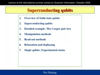
Superconducting qubits
Superconducting qubits. Overview of Solid state qubits Superconducting qubits Detailed example: The Cooper pair box Manipulation methods Read-out methods Relaxation and dephasing Single qubits: Experimental status. 1. Overview of solid state qubits. Solid State Qubits. Energy scales.

Superconducting qubits
E N D
Presentation Transcript
Superconducting qubits • Overview of Solid state qubits • Superconducting qubits • Detailed example: The Cooper pair box • Manipulation methods • Read-out methods • Relaxation and dephasing • Single qubits: Experimental status
Energy scales Atoms and ions Single system Identical systems possible ∆E=> ~500 THz optical frequencies High temperature Hard to scale Solid state systems Single system System taylored ∆E=> ~10 GHz microwave frequencies Low temperature 20mK Potentially scalable NMR-systems Ensemble system Identical systems possible ∆E=> ~100 MHz radio frequencies High temperature Impossible to scale ?
Things to keep in mind • These is a macroscopic system, they typically contains 109 atoms • Thus coherence is hard to keep, relatively short decoherence times • Nanolithography makes the system (relatively) easy to scale • Experimental research on solid state qubits started late compared to other types of qubits
Requirements for read-out systems Two different strategies:Single quantum systems quantum limited detectorsEnsembles of systems normal detectors • Photons Photon detectors (hard for IR and mw) • Magnetic flux SQUIDs • Charge Single Electron Transistors • Single spin (Convert to charge)
Advantages and drawbacks of superconducting systems Advantages Energy gap Protects against low energy exitations Good detectors SQUIDs, SETs Nano lithography Relatively easy scaling Drawbacks ”Large systems” Relatively short decoherence times Cooling The low energies require cooling to <<1K
Superconducting qubit characteristics Which degree of freedomcharge, flux, phase True 2-level systemquasi 2-level system Representation of one qubitsingle system ManipulationMicrowave pulses, rectangular pulses Level splitting~10GHz Type of read-outSquid, SET, dispersive Back action of read outSingle shot possible Operation time 100 ps to 1ns Decoherence time 4 µs obtained Scalabilitypotentially good Coupling between qubitsstatic, tunable, via cavity
Carge versus phase/flux Charge Quantisation on a metalic island Fluxoid Quantisation in a superconducting ring (Josephson) junction Josephson junction Flux Charge Inductance Capacitance Josephson coupling energy EJ Charging energy EC Current Voltage Conductance Resistance
Superconducting qubits charge qubit EJ ~ 0.1 EC Quantronium EJ ~ EC flux qubit EJ ~ 30 EC phase qubit EJ ~ 100000 EC NEC, Chalmers, Yale Saclay, Yale Delft, NTT NIST/Santa Barbara Q and j are conjugate variables which obey the commutation relation: Q well defined well defined
1 0 superposition state Single Cooper-pair tunneling Tunnel junction I1〉 Reservoir -1 SQUID loop 1 1.5 0.5 Gate Box Probe I0〉 The NEC qubit Y. Nakamura et al., Nature 398, 786 (1999).
The quantronium, charge-phase (Saclay) T2≈0.5 µs D. Vion et al., Science 296, 286 (2002)
Jaynes-Cummings Hamiltonian Coupling a qubit to a resonator (Yale) Vacuum Rabi splitting, A. Wallraff, Nature 431 162 (2004)
Ibias E F 2D +Ip Icirc 0 -Ip 0.5 F/Fo Persistent-current qubit (Delft) flux qubit with three junctions & small geometric loop inductance H = hsz + Dsx with h=(F/Fo-0.5) FoIp Science 285, 1036 (1999)
The phase qubit (NIST) Large size ~100µm McDermott et al. Science 307, 1299 (2005)
1.6 E 1.4 C J E / E 1.2 1.0 0.8 0.6 0.4 0.2 n g 0.0 -0.2 0.0 0.2 0.4 0.6 0.8 1.0 1.2 The Single Cooper-pair box (SCB) Charge states degenerate ∆ > EC > EJ > T 2.5K ~1.5K ~0.5K 20mK Likharev and Zorin LT17 (84)
The Single Cooper-pair box (SCB) Which degree of freedom Charge Representation of qubit single circuit Levels multi but uses only the two lowest Manipulation mw- or rectangular- pulses Type of read-out Single Electron Transistor, Josephson junction, dispersive Back action of read out single shot possible, very low for dispersive RO Operation time 100 ps Decoherence time 1µs Scalability Yes Coupling capacitive, or via resonator
How does the SCB work as a Qubit Analogy to a single spin in a magnetic field Shnirman, Makhlin, Schön, PRL, RMP, Nature
E/4EC ng <n> ng Eigenstates and Eigenvalues Eigen values for two state system Eigen states The Coulomb staircase Expectation value for n
Energies, and the optimal point Energy levels Optimal point E/4EC Optimal point The Coulomb staircase <n> Level splitting ng=CgVg/2e At the optimal point the system is insensitive (to first order) to fluctuations in the control parameters ng and
Representation of the Qubit • The basic building block of a quantum computer is called a Qubit • Any two level system which acts quantum mechanically (having quantum coherence) can in principle be used as a Qubit. The Bloch Sphere Ground state Exited state
Manipulation with rectangular pulses t<0 Starting at ng0 t=0 Go to ng0+∆ng t=∆t Go back to ng0 The left sphere with two adjacent pure charge states at the north and south poles corresponds to a CPB with EJ /EC << 1, which is driven to the charge degeneracy point with a fast dc gate pulse. Nakamura et al. Nature (99)
Microwave pulses (NMR-style) The energy eigenstates at the poles described within the rotating wave approximation. The spin is represented by a thin arrow whereas fields are represented by bold arrows. The dotted lines show the spin trajectory, starting from the ground state. NMR-like Control of a Quantum Bit Superconducting Circuit E. Collin, et al. Phys. Rev. Lett., 93, 15 (2004).
Comparing the two methods Microwave pulses Slower, typical π pulse Timing is easier, NMR techniques can be used Smaller amplitude and monocromatc More gentle on the environment Works at the optimal point Rectangular pulses Faster, typical π pulse More accurate timing required Large amplitude and wide frequency content Shakes up the environment Can not stay at optimal point
-e -e + probe • detect the state as current • initialize the system to Read-out with a probing junction (NEC) • Josephson-quasiparticle cycle Fulton et al. PRL ’89 -2e Cooper-pair box Repeted measurement gives a current
1 0 superposition state Single Cooper-pair tunneling Tunnel junction I1〉 Reservoir -1 SQUID loop 1 1.5 0.5 Gate Box Probe I0〉 The NEC qubit Y. Nakamura et al., Nature 398, 786 (1999).
Read-out with SET sample and hold (NEC) Manipulation Trap quasi particles Measure trap with SET Single shot, but still fairly slow Measurement circuit is electrostatically decoupled from the qubit Final states are read out after termination coherent state manipulation
time pulsed bias current ~ 5 ns rise/fall time tmeas~5 ns,ttrail~500 ns Switching quantum operations reference trigger V Vthr I V 1 0 0 time 9 0 0 8 7 0 switching probability (%) 6 0 5 0 4 0 3 0 0 2 0 1 0 2 . 3 2 . 4 2 . 5 2 . 6 2 . 7 p u l s e h e i g h t @ A W g e n e r a t o r ( V ) pulse height Switching SQUID readout scheme (Delft) each readout only two possible outputs pulse height adjusted for ~50% switching SQUID switched to gap voltage probability measured with ~ 5000 readouts SQUID still at V=0 Room temp. output signal
A single Cooper-pair box qubit (Chalmers)integrated with an RF-SET Read-out system A two level systen based on the charge states |1> = One extra Cooper-pair in the box |0> =No extra Cooper-pair in the box Büttiker, PRB (86) Bouchiat et al. Physica Scripta (99) Nakamura et al., Nature (99) Makhlin et al. Rev. Mod. Phys. (01) Aassime, PD et al., PRL (01) Vion et al. Nature (02) ∆ >> EC >> EJ(B) >> T 2.5K 0.5-1.5K 0.05-1K 20mK
Vdc Vac The Radio-Frequency Single Electron Transistor (RF-SET) Very high speed: 137 MHz R. Schoelkopf, et al. Science 280 1238 (98) Charge sensitivity: ∂Q= 3.2 µe/√Hz A. Aassime et al. APL 79, 4031 (2001) Current Voltage characteristics Modulation of conductance and reflection
Performance of the RF-SET Frequency domain: ∂Q=0.035erms, fg=2MHz Time domain: ∆Q=0.2e, inset 0.05e Results: Aassime et al. Charge sensitivity: ∂Q= 3.2 µe/√Hz APL 79, 4031 (2001) Energy sensitivity: ∂e = 4.8 h PRL 86, 3376 (2001)
Coupling a qubit to a resonator (Yale) A. Wallraff, Nature 431 162 (2004)
The Cooper-pair box as a Parametric Capacitance We define an effective capacitance which contains two parts At the degeneracypoint we get: Büttiker, PRB (86) Likharev Zorin, JLTP (85) c.f. the parametric Josephson inductance
Disspative part, R Reactive part, C (or L) Quadrature measurements with the RF-SET Cooper-pair transistor similar to Cooper-pair box High speed: 137 MHz Schoelkopf, et al. Science (98) Charge sensitivity: ∂Q= 3.2 µe/√Hz Aassime et al. APL 79, 4031 (2001)
J1 DJQP J2 Drain -3, -1 Source -1, 1 Drain -1, 1 Source 0, 2 The Josephson Quasiparticel cycle: JQP Phase response Cooper-pair resonance Quasi part transition One junction is resonant part of the time Quasi part transition Cooper-pair resonance
Source jcn in resonance Drain jcn in resonance The Double Josephson Quasiparticle cycle: DJQP Drain -3, 1 Source -1, 1 Drain -1, 1 Source 0, 2 One junction is always resonant but only one at the time This results in an average CQ
Quantitative Comparison of the Quantum Capacitance If the phase shift is small it can be approximated by: Assuming equal capacitances we can calculate CQ for a two level system and compare with the data. T=140 mK From spectroscopy EJ/EC=0.12 Temperature adds to the FWHM
Junction 1 Junction 2 Spectroscopy on the quantum capacitance By tuning only one junction into resonance we can excite the system to the exited state, which has a capacitance of the opposite sign P= Probability to be in the exited state EJ1=3.0 GHz EJ2=2.8 GHz
Cc Cin CT Cg Quantum Cap Qubit • Operate and readout at optimal point • No intrinsic dissipation • Tank circuit protects qubit by filtering environment • Lumped element version of Yale cavity experiment, Wallraff et al. Nature (04)
The Coulomb Staircase Comparingthe Normal and the Superconducting State 2e periodicity is achieved if Ec is sufficiently small <1K Bouchiat et al. Physica Scripta (98) Aumentado et al. PRL (04) Gunnarsson et al. PRB (04)
The Coulomb staircase comparingthe normal and the superconducting state Small step occures due to quasi particle poisoning Bouchiat et al. Physica Scripta (98)