Data Flow Analysis 4 15-411 Compiler Design
E N D
Presentation Transcript
Data Flow Analysis 415-411 Compiler Design Nov. 8, 2005
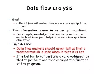
Example from last time Nodes represent sequences of instructions with no branches. Edges represent control flow between nodes.
Constant Propagation • Convenient to associate a pool of propagated constants with each node in the graph. • Pool is a set of ordered pairs which indicate variables that have constant values when node is encountered. • The pool at node B denoted by PB consists of a single element (a,1) since the assignment a:= 1 must occur before B.
Constant Pools • Let V be a set of variables, C be a set of constants, and N be the set of nodes in the graph. • The set U = V £ C represents ordered pairs which may appear in any constant pool. • All constant pools are elements of the power set U, denoted P(U).
Constant Propagation (cont.) • Fundamental problem of constant propagation is to determine the pool of constants for each node in a program graph. • By inspection of the program graph for the example, the pool of constants at each node is • PA = PB = {(a, 1)} PC = {(a, 1)} PD = {(a, 1), (b, 2)} • PE = {(a, 1), (b, 2), (d, 3)} PF = {(a, 1), (b, 2), (d, 3)}
Constant Propagation (cont.) • PN may be determined for each node N in the graph as follows: • Consider each path (A, p1,p2, …, pn,N). Apply constant propagation along path to obtain set of constants at node N. • Intersection for each path to N is the set of constants which can be assumed for optimization. • (It is unknown what path will be taken at execution time, so intersection is conservative choice)
Constant Propagation (cont.) • Successively longer paths from A to D can be evaluated, resulting in PD,3 , PD,4 , …, PD,nfor arbitrarily large n. • The pool of constants that can be assumed no matter what flow of control occurs is the set of constants common to all PD,i , i.e. • Åi PD,i • This procedure is not effective since the number of such paths may have no finite bound, and the procedure would not halt.
Optimizing Function for Constant Propagation • It is useful to define an optimizing functionf which maps an input pool together with a particular nodeto a new output pool. • The optimizing function for constant propagation is • f: N £P(U) !P(U) • where (v, c) 2 f(N, P) if and only if • 1. (v, c) 2 P and the operation at node N does not assign a new value to the variable v. • 2. The operation at N assigns an expression to the variable v, and the expression evaluates to the constant c.
Optimization Function for Example • The optimizing function can be applied to node A with an empty constant pool resulting in • f(A, ; ) = {(a,1)}. • The function can be applied to B with {(a, 1)} as the constant pool yielding • f(B, {(a, 1)}) = {(a, 1), (c, 0)}.
Extending f to Paths in the Graph • Given a path from entry node A to an arbitrary node N, optimizing pool for path is determined by composing the function f. • For example, f(C, f(B, f(A, ;))) = {(a, 1), (c, 0), (b, 2)} is the constant pool for D for this path. • Sometimes the notation is cleaner to write • fC (fB (fA ())) or fC± fB± fA ().
Computing the Pool of Optimizing Information. • The pool of optimizing information which can be assumed at node N in the graph, independent of the path taken at execution time, is • PN = Å {x | x 2 FN}. • Here FN = { f(pn, f(pn-1, …, f(p1, P))…)| (p1, p2, …, pn, N) is a path from an entry node p1 with corresponding entry pool P to node N}.
Lattices • A partial order is a lattice if u andt are defined so that • u is the meet or greatest lower bound operation • x u y · x and x u y · y • If z · x and z · y then z · x u y • t is the join or least upper bound operation • x · x t y and y · x t y • If x · z and y · z, then x t y · z
Lattices (cont.) • A finite partial order is a lattice if meets and joins exist for every pair of elements • A lattice has unique elements bot and top such that • x u? = ? x t? =x • x u> = x x t> = > • In a lattice • x · y iff x u y = x • x · y iff x t y = y
Monotonicity • A function f on a partial order is monotonic if and only if • x · y implies f(x) · f(y) • Can show that optimizing function f: N £P(U) !P(U) for constant propagation is monotonic in its second argument.
Distributive Data Flow Problems • By monotonicity, we also have • A function f is distributive or has the homomorphism property if
Benefit of Distributivity • Joins lose no information
Accuracy of Data Flow Analysis • Ideally, we would like to compute the meet over all paths (MOP) solution: • Let fi be the transfer function for statement si • If p is a path {s1, ..., sn}, let fp= fn± fn-1±...± f1 • Let path(s) be the set of paths from the entry to s • If a data flow problem is distributive, then solving data flow equations in the standard way yields the MOP solution
What Problems are Distributive? • Analyses of how the program computes • Live variables • Available expressions • Reaching definitions • Very busy expressions • All Gen/Kill problems are distributive
A Non-Distributive Example • Constant propagation • In general, analysis of what the program computes is not distributive
Constant Propagation and the Homomorphism Prop. • Does the Optimizing function for Constant Propagation satisfy the homomorphism? • F(1, ) = {(x,1)} • P1= F(2, F(1,)) = {(x, 1), (y, 2)} • F(3, P) = {(x, 2)) • P2 = F(4, F(3,)) = {(x, 2), (y, 1)} • F(5, P1Å P2) = F(5,) = • F(5, P1)) = {(x, 1), (y, 2), (z, 3)} • F(5, P2)) = {(x, 2), (y, 1), (z, 3)} • F(5, P1) Å F(5, P2) = {(z, 3)} = F(5, P1Å P2)
Undecidability of MOP Problem • Surprise!! • The MOP problem is undecidable for Constant Propagation. • No algorithm exists to compute the MOP solution for all instances of the constant propagation problem.
Meet-Semilatticies • Let the finite set L be the set of all possible optimizing pools for a given application. • Let ube a meet operation with the properties: • u : L£L!L • x u y = y u x • x u (y u z) = (x u y) u z • where x, y z 2L. The set L and the uoperation define a finite meet-semilattice.
Ordering on Meet-Semilattices • The u operation defines a partial ordering on L by • x 6 y if and only if x u y = x. • Similarly, • x < y if and only if x 6y and x y.
Monotone Data Flow Analysis Frameworks • A monotone data flow analysis framework is a triple D= (L, u ,F) where • (L, u) is a semilattice of finite length with zero element 0, and • F is a monotone operation space associate with L.
Monotone Operation Spaces • Let (L, u) be a semilattice of finite length with a zero element. • A set of operations F on L is said to be a monotone operation space associated with L iff the following conditions hold: • Each f 2 F is monotonic, i.e., • (8 x, y 2 L)[x 6 y implies that f(x) 6 f(y)]. • 2. There exists an identity operation e in F, i.e. • (9 e 2 F) (8 x 2 L) [e(x) = x] • 3. F is closed under composition, i.e., (8 f, g 2 F)[f ± g 2 F] • 4. For each x 2 F there exists an f 2 F such that x = f(0).
Distributive Frameworks • A monotone framework D = (L,u,F) is called a distributive framework if and only if • (8 f 2 F) (8 x, y 2 L) [f(x u y) = f(x) u f(y)]. • This really just the homomorphism property mentioned earlier.
Maximum Fixpoint Solution (MFP) • Let I = (G, M) be an instance of a monotone framework D = (L, u, F). • Let fi(P) be the operation associated with node i, and let the nodes of G be numbered from 2 to n by rPostorder. • The maximum fixed point (MFP) solution of I is defined as the maximum fixed point of the following equations. • x1 = 0, xi =u j2 pred(i) fj (xj) for 2 6 i 6 n.
Conditions for Algorithm • If X ½L, the generalized meet operation uX is defined as the pairwise application of u to the elements of X. • Lis assumed to have a “zero element” 0 such that 0 6 x for all x 2L. • An augmented set L’ is constructed from L by adding a “unit element” 1 such that 1 is not in L and 1 Æ x = x for all x in L. • The set L’ = L[ {1}. It follows that x <1 for all x in L.
Conditions for Algorithm (cont.) • Need an “optimizing function” f: N£L!L . • It should have the distributive or homomorphism property: • F(N, x Æ y) = f(N, x) Æ f(N, y) for all N 2N and x, y 2L. • Note that f(N, x) < 1 for all N 2N and x 2L.
Global Analysis Algorithm • Global analysis starts with an entry pool set EP½I£L, where (e, x) 2EP if e 2I is an entry node with optimizing pool x 2L. • A1 [initialize] L := EP. • A2 [terminate ?] If L = ; then halt. • A3 [select node] Let L’ 2 L, L’ = (N, Pi) for some N 2N and Pi2L. • Then L := L – {L’}. • A4 [Traverse] Let PN be the current approximate pool for node N • (Initially PN = 1). If PN6 Pi the go to step A2. • A5 [set pool] PN := PNÆ Pi, L:= L [ {(N’, f(N, PN)) | N’ 2 I(N)}. • A6 [Loop] Go to step A2.
MOP vs. MFP Solutions • Kildall provided a general iterative algorithm for distributive frameworks (see previous slide). • He proved that his algorithm converges to the MFP solution of a distributive framework and that for distributive frameworks the MFP solution is equal to the MOP solution. • Kam and Ullman proved that when Kildall’s iterative algorithm is applied to a monotone framework, it converges to the MFP solution of that framework.