Download
1 / 20
200 likes | 394 Vues
September 2006. Bayesian methods for parameter estimation and data assimilation with crop models. David Makowski and Daniel Wallach INRA, France. Objectives of this course. Introduce basic concepts of Bayesian statistics. Describe several algorithms for estimating crop model parameters.

E N D
September 2006 Bayesian methods for parameter estimation and data assimilation with crop models David Makowski and Daniel Wallach INRA, France
Objectives of this course • Introduce basic concepts of Bayesian statistics. • Describe several algorithms for estimating crop model parameters. • Provide the readers with simple programs to implement these algorithms (programs for the free statistical software R). • Show how these algorithms can be adapted for data assimilation. • Present case studies.
Organisation • Part 1: First steps in Bayesian statistics. • Part 2: Likelihood function and prior distribution. • Part 3: Parameter estimation by importance sampling. • Part 4: Parameter estimation using MCMC methods. • Part 5: Bayesian methods for data assimilation.
Some references Bayes, T. 1763. An essay towards solving a problem in the doctrine of chances. Philos. Trans. Roy. Soc. London, 53, 370-418. Reprinted, with an introduction by George Barnard, in 1958 in Biometrika, 45, 293-35. Carlin, B.P. and Louis, T.A. 2000. Bayes and empirical Bayes methods for data analysis. Chapman & Hall, London. Chib, S., Greenberg, E. 1995. Understanding the Metropolis-Hastings algorithm. American Statistician 49, 327-335. Gelman A., Carlin J.B., Stern H.S., Rubin D. 2004. Bayesian data analysis. Chapman & Hall, London. Gilks, W.R., Richardson, S., Spiegelhalter, D.J. 1995. Markov Chain Monte Carlo in practice. Chapman & Hall, London. Robert, C. P., Casella, G. 2004. Monte Carlo Statistical Methods. Springer, New York. Smith, A. F. M., Gelfand, A. E. 1992. Bayesian statistics without tears: A sampling-resampling perspective. American Statistician 46, 84-88. Van Oijen, M., Rougier, J, Smith, R. 2005. Bayesian calibration of process-based forest models: bridging the gap between models and data. Tree Physiology 25, 915-927. Wallach D., Makowski D., Jones J. Working with dynamic crop models. Evaluation, Analysis, Parameterization and applications. Elsevier, Amsterdam.
Part 1: First steps in Bayesian statistics General characteristics • The Bayesian approach allows one to combine information from different sources to estimate unknown parameters. • Basic principles: • - Both data and external information (prior) are used. • Computations are based on the Bayes theorem. • Parameters are defined as random variables.
Part 1: First steps in Bayesian statistics Notions in probability • Statistics is based on probability theory. • Basic notions in probability are needed to apply Bayesian methods: • Joint probability. • Conditional probability. • Marginal probability. • Bayes theorem.
Part 1: First steps in Bayesian statistics Joint probability • Consider two random variables A and B representing two possible events. • Joint probability = probability of event A and event B. • Notation: P(AB) or P(A, B).
Part 1: First steps in Bayesian statistics Example 1 A = rain on January 1 in Toulouse (possible values: « yes », « no »). B = rain on January 2 in Toulouse (possible values: « yes », « no »). P( A=yes, B=yes): Probability that it rains on January 1 AND January 2.
Part 1: First steps in Bayesian statistics Conditional probability • Consider two random variables A and B representing two possible events. • Conditional probability = probability of event B given event A. • Notation: P(B | A).
Part 1: First steps in Bayesian statistics Example 1 (continued) A = rain on January 1 in Toulouse (possible values: « yes », « no »). B = rain on January 2 in Toulouse (possible values: « yes », « no »). P( B=yes | A=yes): Probability that it rains on January 2 GIVEN that it rained on January 1.
Part 1: First steps in Bayesian statistics Marginal probability • Consider two random variables A and B representing two possible events. • Marginal probability of A = probability of event A • Marginal probability of B = probability of event B • Notation: P(A), P(B).
Part 1: First steps in Bayesian statistics Example 1 (continued) A = rain on January 1 in Toulouse (possible values: « yes », « no »). B = rain on January 2 in Toulouse (possible values: « yes », « no »). P( A=yes) = Probability that it rains on January 1. P(A=no) = Probability that it does not rain on January 1
Part 1: First steps in Bayesian statistics Relationships between probabilities Expression for joint probability P(A,B) = P(B,A) = P(B|A)P(A) = P(A|B)P(B) Expression for marginal probability P(B) = ΣiP(B|A=ai)P(A=ai) P(A) = ΣiP(A|B=bi)P(B=bi)
Part 1: First steps in Bayesian statistics Bayes theorem Bayes’ theorem allows one to relate P(B | A) to P(B) and P(A|B). P(B | A) = P(A | B) P(B) / P(A) This theorem can be used to calculate the probability of event B given event A. In practice, A is an observation and B is an unknown quantity of interest.
Part 1: First steps in Bayesian statistics Example 2 A woman is pregnant with twins, two boys. Probability that the twins are identical ? A = sexes of the twins (possible values: « boy, girl », « girl, boy », « boy, boy », « girl, girl »). B = twin type (possible values: « identical », « not identical »). The value of A is known but not the value of B. P(B=identical | A=two boys) ?
Part 1: First steps in Bayesian statistics Example 2 (continued) Bayes’ theorem: P(B=identical | A=two boys)= P(A=two boys | B=identical) P(B=identical)/P(A=two boys) Numerical application: Prior knowledge about B P(B=identical)=1/3 P(A=two boys) = 1/3 P(A=two boys | B=identical) = 1/2 P(B=identical | A=two boys) = 1/2 *1/3 / 1/3 = 1/2
Part 1: First steps in Bayesian statistics Bayes’ theorem for model parameters θ: vector of parameters. y: vector of observations P(θ): prior distribution of the parameter values. P(y| θ): likelihood function. P(θ| y): posterior distribution of the parameter values. often difficult to compute
Part 1: First steps in Bayesian statistics How to proceed for estimating the parameters of models ? We proceed in three steps: Step 1: Definition of the prior distribution. Step 2: Definition of the likelihood function. Step 3: Computation of the posterior distribution using Bayes’ theorem.
Next Part Forthcoming: - the notions of « likelihood » and of « prior distribution ». - applications to solve agronomic problems.