Status of 3D track-finding

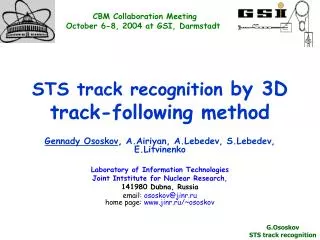
CBM Collaboration Meeting October 6-8, 2004 at GSI, Darmstadt Status of 3D track-finding Gennady Ososkov, A.Airiyan, A.Lebedev, S.Lebedev Laboratory of Information Technologies Joint Intstitute for Nuclear Research, 141980 Dubna, Russia email: ososkov@jinr.ruhome page: www.jinr.ru/~ososkov G.Ososkov Status of 3D track-finding

Remindering The track recognition procedure was accomplished in 3D space on both X-Z and Y-Z projections simultaneously by alternating between both views predicting a track position on the next station and searching for hits in the vicinity of the predicted position. However this approach was oriented on the earlier designed STS with hybrid pixel detectors (HPD) and scarcely would suit for the MAPS or Si-strip detectors. Two scenarios are (still) possible: 1. Maps for 1-3 stations and Si-strip for 4-7 stations; 2. HPD and Si-strip. In the first case both types of detectors need a guidance. In the 2d case HPD data can be handled by 3D track-following and, if necessary, provide a guidance for the robust track search and fitting in the Si-strip STS section. Let us consider, at first, the second scenario. What’s new was done Y-Z and X-Z projections of an event. Hits are marked as blue points

Stage 1. Starting from the middle of the target area we connect this point sequentially with all points on the first station in Y-Z view, where tracks are close to straight lines. Each time we prolong the straight line driven via these two points to the plane of the second station. Then we set aside from the crossing point an asymmetrical corridor and look for all points appeared in this corridor. For each of these found points and two more on the previous stations we draw in X-Z view a parabola to estimate Pxz - the momentum projection at the 3-d station. Then taking the magnetic field into account we use the corresponding curvature radius r for a new parabolic prolongation to the crossing with the next station plane. Since several prolongations can happened, we set aside corridors from each of pointpredicted matching found points in both X-Z and Y-Z views. Prediction and search in YoZ view Prediction and search in XoZ view

How to take the magnetic field into account Knowing parametera from the initial parabola x=az2+bz+cwe obtain the approximate value of Pxz for the 2d station asPxz =0.052+0.00134/|a|. We use approximations previously calculated for each station by MC-data. From Pxz and the Y-component By of magnetic field known from its map we obtain the approximation of the curvature radius r = Pxz /0.3*Byat the point (x2,z2), in which we also know the tangent slope tgα=2a*z2+b. That’s enough to draw a new parabola to make a prediction on the 3d station. Further prolongations are made in the same manner. The next trick consists in very careful preliminary calculations of tables with confidence bounds of prediction corridors depending on the station numberand thesign of the particle charge. Those tables were calculated by statistics obtained by many thousands simulated events. Pxz versus parabola parameter a for the 3d station.Distribution and approximation

Since the conventional approach to use symmetrical 3σcorridors had failed being too inefficient, we use the distributions of deviations between real hit positions and their predictions for the all remaining stations. Magnetic field knowledge gave us a striking result: distributions and corresponding confidential corridors for prediction got narrowed 6 times. That increases substantially the accuracy of prediction and speed up track-finding performance. Stage 2.Having tracks found on the first stage we make a selection on the basis of the following criterion: each point can belong to the only one track. So any track with one or more points belonging to some other track must be rejected. Unlike to 70% criterion of efficiency, when a reconstructed track is assigned to a generated particle if at least 70% of its hits have been caused by this particle, we use 100% criterion of efficiency in order to reduce the ghost rate. Without taking magnetic field into account it was in average 92% with 1.62 ghosts per event for 6&7 hit tracks.

Si-strip STS section peculiarities has been studied on a sample ofspace points with their ΔX and ΔY errors. 2D histograms of those errors are as follows: RMS grows with the station number not exceeding 36 mkm Since these space points are not provided by any information about track hits in the first three stations, we tried to simulate Si-strip hits by smearing GEANT hits adding normally distributed random numbers with zero mean and σ=36 mkm, while on the first three station hits were smeared with σ=10 mkm.

Despite of this smearing the obtained track-finding efficiency is not worse than it was without taking the magnetic field into account (92% in average). Efficiency rate with 100% criterion and taking the magnetic field into account Vertex positioning improvement.Although the algorithm has shown its stability to minor vertex shifts, the option exists to estimate the vertex position after the first run on the basis of several reference tracks. Then in the second run all track-following process is recalculated with the improved vertex position.

The 1st scenario. Elastic arm methods can help The idea of "elastic" methods (elastic tracking, elastic arms, deformable templates) is based on known parametric form of curves to be recognized and consists in a simultaneous accomplishment of both stages: a curve recognition and fitting.Proposing the elastic tracking method, Gyulassy and Harlander (G & H, 1991) based on the concept of the elastic template, i.e. the track equation depending on varying parameters so that being bent with their variations, a curve described by this equation passed as close as possible to the points measured in a track. This approach can physically be described as interaction between the positively charged template and negatively charged spatial points measured in the track. The better the elastic template fits points, the lower the energy of their interaction. Let a charge of the track template be distributed with the density ρT(r), and the set of measured points have charge density ρ(r’). Calculating the energy E of interaction between these two charges, we obtain where V is the Lorentz potentialwith the time-dependent width T is the time constant, a is the maximal distance, at which points are still accredited to this template, and b~σres is spatial resolution of a detector. It is evident that b << a .

Taking measurement discreteness into account, we obtain the track interaction energy as the sum: were, N is the number of points in the track, xi and r are the i-th point measured in the space and its distance from the template, respectively, and is the set of the track parameters. When a detector is placed in a homogeneous magnetic field, the track is described by a helix with the curvature κ , helix angle λ, and phase Φat the point xi , i.e. . The functional E(π,t) depends on the points of only one track. Although all tracks could be fitted simultaneously, G&H did not recommend such a synchronous fit. To avoid E(π,t) getting caught in local spurious minima the simulated annealing procedure is applied. On the first iteration w(t) is taken for the highest temperature, when E(π,t) has the only one minimum. Then w(t) is narrowed gradually allowing more and more accurate search of the global minimum.

Elastic templates as robust tracking Let us consider linear track model: xi= x0 + txzi + εi i= 1,…,n; where zi is z-coordinate of i-th plane, xi is the only measured point at this i-th plane, εi is a measurementerror supposed to be normally distributed εi€N(0;σ ). Two simple examples, when Least Squareapproach L(p) = Σiεi2→minp (1) does not work: a) point - outlier b) uniform contamination In both cases the crucial assumption of residual normality is violated - it demands to replace the Least Square functional Σiεi2by a functional L(p,σ)=Σiρ(εi )(2) where εi areresiduals and ρ(ε) is a compact contribution function

It’s easy to show that for minimizing of the functional (2) by parameters its derivative by denoting can be modified to the form which is similar to the normal LSM equations, but with replacement of the numerical weight coefficients to the weight function w(ε)to be recalculated on each step of an iterative procedure. It gives a weight to each measured poit depending on its distance εfrom the fitted curve. Weight function must quickly decrease with growing the residual ε Arisen problems: 1. Lack of theoretical foundation for the use of w(ε) 2. Initial values of parameters to start iterations 3. Computational problems due to non-uniqueness of the solution 4. Helix applications

Lack of theoretical foundations for w(ε) Let us return to Si-strip ΔX and ΔY distribution. Fake contamunations look uniformal Our proposalfor such a case of the uniform contamination : use the residual distribution model as a mixture of two distributions: gaussian φ(ε)and the uniform oneh(ε) = h0 f(ε) = (1-c) φ(ε) + c h(ε) to evaluate the corresponding likelihood equation (2) in order to derive the optimal weights w(ε) 2D histogram of all ΔX and ΔY in linear scale with the only parameter , whichis determined by the contamination of data not in the whole range of the sample but within its essential part where all useful observations are practically concentrated. Now the next problem is Initial values of parameters to start iterations

The 1st scenario. Hough transform & robust elastic tracking The Hough transform is needed to get starting parameters for robust iterations Helix parametrization to initialize a track. Using unique combinations of all sub-sets of 3 hits, helix parameters can be calculated analytically since a set of three hits is sufficient to determine the parameters for a helix: curvature (κ=1/R), dip angle (λ) and phase (Φ), what is possible determine by a 3D Hough transform (or 2D & 1D sequentially). X(s)=x0+1/k[cos(Φ0 +h s cosλ) - cosΦ0) Z(s)=z0+1/k[sin(Φ0 +h s cosλ) - sinΦ0) Y(s)=y0+s sinλ, where s is the path length along the helix, (x0,y0,z0) is the vertex coord. at s=0, Φ0 is its azimut angle of the starting point (phase): Ф0 =Ψ - h π/2=arctan((x1-xc)/(z1-zc)) By is the y component of the field q is charge of the particle in units of positron charge h is the sense of rotation of the projected helix in the xy-plane, i.e. h = -sign(qB) = +-1 Then the momentum can be evaluated as:

What to do next (not, of course, by only Dubna group) 1. Organize a rough estimation of Si-strip track parameters by 3D Hough transform. 2. Robust track finding 3. Apply found tracks to facilitate tracking in the MAPS STS section. A proposal of the robust approach to Si-stip STS track finding Now we consider track-finding problem as finding minima to the functional L(p,t)=∑w(di)di2, where di is the Euclidean distance between the space point i and the template and p is the set of track parameters p={κ,λ,Φ,(x0,y0,z0)}. Again using the dependence of the curvature from the magnetic field one can make corrections calculating the distance from the current point to the helix. Robust weights are to be recalculated iteratively during the minimization process. Their functional view is to be selected depending on the behaviour of the ΔX and ΔY distributions. It could be approximated by a mixture of gaussian with some distribution generated by fake points: either uniform of very wide gaussian distribution. Simulated annealing schedule should allow to avoid local minima

Status of 3D track-finding