Table of Contents Chapter 14 (Queueing Models)
910 likes | 1.41k Vues
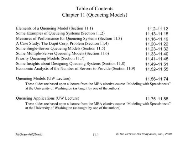
Elements of a Queueing Model (Section 14.1) 14.2–14.13 Some Examples of Queueing Systems (Section 14.2) 14.14–14.16 Measures of Performance for Queueing Systems (Section 14.3) 14.17–14.20 A Case Study: The Dupit Corp. Problem (Section 14.4) 14.21–14.23

Table of Contents Chapter 14 (Queueing Models)
E N D
Presentation Transcript
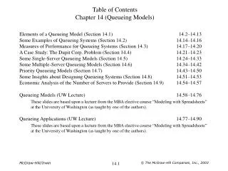
Elements of a Queueing Model (Section 14.1) 14.2–14.13 Some Examples of Queueing Systems (Section 14.2) 14.14–14.16 Measures of Performance for Queueing Systems (Section 14.3) 14.17–14.20 A Case Study: The Dupit Corp. Problem (Section 14.4) 14.21–14.23 Some Single-Server Queueing Models (Section 14.5) 14.24–14.33 Some Multiple-Server Queueing Models (Section 14.6) 14.34–14.42 Priority Queueing Models (Section 14.7) 14.43–14.50 Some Insights about Designing Queueing Systems (Section 14.8) 14.51–14.53 Economic Analysis of the Number of Servers to Provide (Section 14.9) 14.54–14.57 Queueing Models (UW Lecture) 14.58–14.76 These slides are based upon a lecture from the MBA elective course “Modeling with Spreadsheets” at the University of Washington (as taught by one of the authors). Queueing Applications (UW Lecture) 14.77–14.90 These slides are based upon a lecture from the MBA elective course “Modeling with Spreadsheets” at the University of Washington (as taught by one of the authors). Table of ContentsChapter 14 (Queueing Models) © The McGraw-Hill Companies, Inc., 2003
A Basic Queueing System © The McGraw-Hill Companies, Inc., 2003
Herr Cutter’s Barber Shop • Herr Cutter is a German barber who runs a one-man barber shop. • Herr Cutter opens his shop at 8:00 A.M. • The table shows his queueing system in action over a typical morning. © The McGraw-Hill Companies, Inc., 2003
Arrivals • The time between consecutive arrivals to a queueing system are called the interarrival times. • The expected number of arrivals per unit time is referred to as the mean arrival rate. • The symbol used for the mean arrival rate is l = Mean arrival rate for customers coming to the queueing system where l is the Greek letter lambda. • The mean of the probability distribution of interarrival times is 1 / l = Expected interarrival time • Most queueing models assume that the form of the probability distribution of interarrival times is an exponential distribution. © The McGraw-Hill Companies, Inc., 2003
Evolution of the Number of Customers © The McGraw-Hill Companies, Inc., 2003
The Exponential Distribution for Interarrival Times © The McGraw-Hill Companies, Inc., 2003
Properties of the Exponential Distribution • There is a high likelihood of small interarrival times, but a small chance of a very large interarrival time. This is characteristic of interarrival times in practice. • For most queueing systems, the servers have no control over when customers will arrive. Customers generally arrive randomly. • Having random arrivals means that interarrival times are completely unpredictable, in the sense that the chance of an arrival in the next minute is always just the same. • The only probability distribution with this property of random arrivals is the exponential distribution. • The fact that the probability of an arrival in the next minute is completely uninfluenced by when the last arrival occurred is called the lack-of-memory property. © The McGraw-Hill Companies, Inc., 2003
The Queue • The number of customers in the queue (or queue size) is the number of customers waiting for service to begin. • The number of customers in the system is the number in the queue plus the number currently being served. • The queue capacity is the maximum number of customers that can be held in the queue. • An infinite queue is one in which, for all practical purposes, an unlimited number of customers can be held there. • When the capacity is small enough that it needs to be taken into account, then the queue is called a finite queue. • The queue discipline refers to the order in which members of the queue are selected to begin service. • The most common is first-come, first-served (FCFS). • Other possibilities include random selection, some priority procedure, or even last-come, first-served. © The McGraw-Hill Companies, Inc., 2003
Service • When a customer enters service, the elapsed time from the beginning to the end of the service is referred to as the service time. • Basic queueing models assume that the service time has a particular probability distribution. • The symbol used for the mean of the service time distribution is 1 / m = Expected service timewhere m is the Greek letter mu. • The interpretation of m itself is the mean service rate.m = Expected service completions per unit time for a single busy server © The McGraw-Hill Companies, Inc., 2003
Some Service-Time Distributions • Exponential Distribution • The most popular choice. • Much easier to analyze than any other. • Although it provides a good fit for interarrival times, this is much less true for service times. • Provides a better fit when the service provided is random than if it involves a fixed set of tasks. • Standard deviation: s = Mean • Constant Service Times • A better fit for systems that involve a fixed set of tasks. • Standard deviation: s = 0. • Erlang Distribution • Fills the middle ground between the exponential distribution and constant. • Has a shape parameter, k that determines the standard deviation. • In particular, s = mean / (k) © The McGraw-Hill Companies, Inc., 2003
Standard Deviation and Mean for Distributions © The McGraw-Hill Companies, Inc., 2003
Labels for Queueing Models To identify which probability distribution is being assumed for service times (and for interarrival times), a queueing model conventionally is labeled as follows: Distribution of service times — / — / — Number of Servers Distribution of interarrival times The symbols used for the possible distributions areM = Exponential distribution (Markovian)D = Degenerate distribution (constant times)Ek = Erlang distribution (shape parameter = k)GI = General independent interarrival-time distribution (any distribution)G = General service-time distribution (any arbitrary distribution) © The McGraw-Hill Companies, Inc., 2003
Summary of Usual Model Assumptions • Interarrival times are independent and identically distributed according to a specified probability distribution. • All arriving customers enter the queueing system and remain there until service has been completed. • The queueing system has a single infinite queue, so that the queue will hold an unlimited number of customers (for all practical purposes). • The queue discipline is first-come, first-served. • The queueing system has a specified number of servers, where each server is capable of serving any of the customers. • Each customer is served individually by any one of the servers. • Service times are independent and identically distributed according to a specified probability distribution. © The McGraw-Hill Companies, Inc., 2003
Examples of Commercial Service SystemsThat Are Queueing Systems © The McGraw-Hill Companies, Inc., 2003
Examples of Internal Service SystemsThat Are Queueing Systems © The McGraw-Hill Companies, Inc., 2003
Examples of Transportation Service SystemsThat Are Queueing Systems © The McGraw-Hill Companies, Inc., 2003
Choosing a Measure of Performance • Managers who oversee queueing systems are mainly concerned with two measures of performance: • How many customers typically are waiting in the queueing system? • How long do these customers typically have to wait? • When customers are internal to the organization, the first measure tends to be more important. • Having such customers wait causes lost productivity. • Commercial service systems tend to place greater importance on the second measure. • Outside customers are typically more concerned with how long they have to wait than with how many customers are there. © The McGraw-Hill Companies, Inc., 2003
Defining the Measures of Performance L = Expected number of customers in the system, including those being served (the symbol L comes from Line Length). Lq = Expected number of customers in the queue, which excludes customers being served. W = Expected waiting time in the system (including service time) for an individual customer (the symbol W comes from Waiting time). Wq = Expected waiting time in the queue (excludes service time) for an individual customer. These definitions assume that the queueing system is in a steady-state condition. © The McGraw-Hill Companies, Inc., 2003
Relationship between L, W, Lq, and Wq • Since 1/m is the expected service timeW = Wq+ 1/m • Little’s formula states thatL = lWandLq= lWq • Combining the above relationships leads toL = Lq + l/m © The McGraw-Hill Companies, Inc., 2003
Using Probabilities as Measures of Performance • In addition to knowing what happens on the average, we may also be interested in worst-case scenarios. • What will be the maximum number of customers in the system? (Exceeded no more than, say, 5% of the time.) • What will be the maximum waiting time of customers in the system? (Exceeded no more than, say, 5% of the time.) • Statistics that are helpful to answer these types of questions are available for some queueing systems: • Pn = Steady-state probability of having exactly n customers in the system. • P(W ≤ t) = Probability the time spent in the system will be no more than t. • P(Wq ≤ t) = Probability the wait time will be no more than t. • Examples of common goals: • No more than three customers 95% of the time: P0 + P1 + P2 + P3 ≥ 0.95 • No more than 5% of customers wait more than 2 hours: P(W ≤ 2 hours) ≥ 0.95 © The McGraw-Hill Companies, Inc., 2003
The Dupit Corp. Problem • The Dupit Corporation is a longtime leader in the office photocopier marketplace. • Dupit’s service division is responsible for providing support to the customers by promptly repairing the machines when needed. This is done by the company’s service technical representatives, or tech reps. • Current policy: Each tech rep’s territory is assigned enough machines so that the tech rep will be active repairing machines (or traveling to the site) 75% of the time. • A repair call averages 2 hours, so this corresponds to 3 repair calls per day. • Machines average 50 workdays between repairs, so assign 150 machines per rep. • Proposed New Service Standard: The average waiting time before a tech rep begins the trip to the customer site should not exceed two hours. © The McGraw-Hill Companies, Inc., 2003
Alternative Approaches to the Problem • Approach Suggested by John Phixitt: Modify the current policy by decreasing the percentage of time that tech reps are expected to be repairing machines. • Approach Suggested by the Vice President for Engineering: Provide new equipment to tech reps that would reduce the time required for repairs. • Approach Suggested by the Chief Financial Officer: Replace the current one-person tech rep territories by larger territories served by multiple tech reps. • Approach Suggested by the Vice President for Marketing: Give owners of the new printer-copier priority for receiving repairs over the company’s other customers. © The McGraw-Hill Companies, Inc., 2003
The Queueing System for Each Tech Rep • The customers: The machines needing repair. • Customer arrivals: The calls to the tech rep requesting repairs. • The queue: The machines waiting for repair to begin at their sites. • The server: The tech rep. • Service time: The total time the tech rep is tied up with a machine, either traveling to the machine site or repairing the machine. (Thus, a machine is viewed as leaving the queue and entering service when the tech rep begins the trip to the machine site.) © The McGraw-Hill Companies, Inc., 2003
Notation for Single-Server Queueing Models • l = Mean arrival rate for customers = Expected number of arrivals per unit time1/l = expected interarrival time • m = Mean service rate (for a continuously busy server) = Expected number of service completions per unit time1/m = expected service time • r = the utilizationfactor= the average fraction of time that a server is busy serving customers = l / m © The McGraw-Hill Companies, Inc., 2003
The M/M/1 Model • Assumptions • Interarrival times have an exponential distribution with a mean of 1/l. • Service times have an exponential distribution with a mean of 1/m. • The queueing system has one server. • The expected number of customers in the system is L = r / (1 –r) = l / (m– l) • The expected waiting time in the system is W = (1 / l)L = 1 / (m – l) • The expected waiting time in the queue is Wq= W – 1/m = l / [m(m – l)] • The expected number of customers in the queue is Lq= lWq = l2 / [m(m – l)] = r2 / (1 – r) © The McGraw-Hill Companies, Inc., 2003
The M/M/1 Model • Theprobability of having exactly n customers in the system is Pn = (1 – r)rnThus,P0 = 1 – rP1 = (1 – r)rP2 = (1 – r)r2 : : • The probability that the waiting time in the system exceeds t is P(W > t) = e–m(1–r)t for t ≥ 0 • The probability that the waiting time in the queue exceeds t is P(Wq > t) = re–m(1–r)t for t ≥ 0 © The McGraw-Hill Companies, Inc., 2003
M/M/1 Queueing Model for the Dupit’s Current Policy © The McGraw-Hill Companies, Inc., 2003
John Phixitt’s Approach (Reduce Machines/Rep) • The proposed new service standard is that the average waiting time before service begins be two hours (i.e., Wq≤ 1/4 day). • John Phixitt’s suggested approach is to lower the tech rep’s utilization factor sufficiently to meet the new service requirement. Lower r = l / m, until Wq≤ 1/4 day,wherel = (Number of machines assigned to tech rep) / 50. © The McGraw-Hill Companies, Inc., 2003
M/M/1Model for John Phixitt’s Suggested Approach(Reduce Machines/Rep) © The McGraw-Hill Companies, Inc., 2003
The M/G/1 Model • Assumptions • Interarrival times have an exponential distribution with a mean of 1/l. • Service times can have any probability distribution. You only need the mean (1/m) and standard deviation (s). • The queueing system has one server. • The probability of zero customers in the system is P0 = 1 – r • The expected number of customers in the queue is Lq= [l2s2 + r2] / [2(1 – r)] • The expected number of customers in the system is L = Lq + r • The expected waiting time in the queue is Wq= Lq/ l • The expected waiting time in the system is W = Wq+ 1/m © The McGraw-Hill Companies, Inc., 2003
The Values of s and Lqfor the M/G/1 Modelwith Various Service-Time Distributions © The McGraw-Hill Companies, Inc., 2003
VP for Engineering Approach (New Equipment) • The proposed new service standard is that the average waiting time before service begins be two hours (i.e., Wq≤ 1/4 day). • The Vice President for Engineering has suggested providing tech reps with new state-of-the-art equipment that would reduce the time required for the longer repairs. • After gathering more information, they estimate the new equipment would have the following effect on the service-time distribution: • Decrease the mean from 1/4 day to 1/5 day. • Decrease the standard deviation from 1/4 day to 1/10 day. © The McGraw-Hill Companies, Inc., 2003
M/G/1 Model for the VP of Engineering Approach(New Equipment) © The McGraw-Hill Companies, Inc., 2003
The M/M/s Model • Assumptions • Interarrival times have an exponential distribution with a mean of 1/l. • Service times have an exponential distribution with a mean of 1/m. • Any number of servers (denoted by s). • With multiple servers, the formula for the utilization factor becomesr = l / smbut still represents that average fraction of time that individual servers are busy. © The McGraw-Hill Companies, Inc., 2003
Values of L for the M/M/s Model for Various Values of s © The McGraw-Hill Companies, Inc., 2003
CFO Suggested Approach (Combine Into Teams) • The proposed new service standard is that the average waiting time before service begins be two hours (i.e., Wq≤ 1/4 day). • The Chief Financial Officer has suggested combining the current one-person tech rep territories into larger territories that would be served jointly by multiple tech reps. • A territory with two tech reps: • Number of machines = 300 (versus 150 before) • Mean arrival rate = l = 6 (versus l = 3 before) • Mean service rate = m = 4 (as before) • Number of servers = s = 2 (versus s = 1 before) • Utilization factor = r = l/sm = 0.75 (as before) © The McGraw-Hill Companies, Inc., 2003
M/M/s Model for the CFO’s Suggested Approach(Combine Into Teams of Two) © The McGraw-Hill Companies, Inc., 2003
CFO Suggested Approach (Teams of Three) • The Chief Financial Officer has suggested combining the current one-person tech rep territories into larger territories that would be served jointly by multiple tech reps. • A territory with three tech reps: • Number of machines = 450 (versus 150 before) • Mean arrival rate = l = 9 (versus l = 3 before) • Mean service rate = m = 4 (as before) • Number of servers = s = 3 (versus s = 1 before) • Utilization factor = r = l/sm = 0.75 (as before) © The McGraw-Hill Companies, Inc., 2003
M/M/s Model for the CFO’s Suggested Approach(Combine Into Teams of Three) © The McGraw-Hill Companies, Inc., 2003
Comparison of Wq with Territories of Different Sizes © The McGraw-Hill Companies, Inc., 2003
Values of L for the M/D/s Model for Various Values of s © The McGraw-Hill Companies, Inc., 2003
Values of L for the M/Ek/2 Model for Various Values of k © The McGraw-Hill Companies, Inc., 2003
Priority Queueing Models • General Assumptions: • There are two or more categories of customers. Each category is assigned to a priority class. Customers in priority class 1 are given priority over customers in priority class 2. Priority class 2 has priority over priority class 3, etc. • After deferring to higher priority customers, the customers within each priority class are served on a first-come-fist-served basis. • Two types of priorities • Nonpreemptive priorities: Once a server has begun serving a customer, the service must be completed (even if a higher priority customer arrives). However, once service is completed, priorities are applied to select the next one to begin service. • Preemptive priorities: The lowest priority customer being served is preempted (ejected back into the queue) whenever a higher priority customer enters the queueing system. © The McGraw-Hill Companies, Inc., 2003
Preemptive Priorities Queueing Model • Additional Assumptions • Preemptive priorities are used as previously described. • For priority class i (i = 1, 2, … , n), the interarrival times of the customers in that class have an exponential distribution with a mean of 1/li. • All service times have an exponential distribution with a mean of 1/m, regardless of the priority class involved. • The queueing system has a single server. • The utilization factor for the server is r = (l1 + l2 + … + ln) / m © The McGraw-Hill Companies, Inc., 2003
Nonpreemptive Priorities Queueing Model • Additional Assumptions • Nonpreemptive priorities are used as previously described. • For priority class i (i = 1, 2, … , n), the interarrival times of the customers in that class have an exponential distribution with a mean of 1/li. • All service times have an exponential distribution with a mean of 1/m, regardless of the priority class involved. • The queueing system can have any number of servers. • The utilization factor for the servers is r = (l1 + l2 + … + ln) / sm © The McGraw-Hill Companies, Inc., 2003
VP of Marketing Approach (Priority for New Copiers) • The proposed new service standard is that the average waiting time before service begins be two hours (i.e., Wq≤ 1/4 day). • The Vice President of Marketing has proposed giving the printer-copiers priority over other machines for receiving service. The rationale for this proposal is that the printer-copier performs so many vital functions that its owners cannot tolerate being without it as long as other machines. • The mean arrival rates for the two classes of copiers are • l1 = 1 customer (printer-copier) per workday (now) • l2 = 2 customers (other machines) per workday (now) • The proportion of printer-copiers is expected to increase, so in a couple years • l1 = 1.5 customers (printer-copiers) per workday (later) • l2 = 1.5 customers (other machines) per workday (later) © The McGraw-Hill Companies, Inc., 2003
Nonpreemptive Priorities Model forVP of Marketing’s Approach (Current Arrival Rates) © The McGraw-Hill Companies, Inc., 2003
Nonpreemptive Priorities Model forVP of Marketing’s Approach (Future Arrival Rates) © The McGraw-Hill Companies, Inc., 2003
Expected Waiting Times with Nonpreemptive Priorities © The McGraw-Hill Companies, Inc., 2003
The Four Approaches Under Considerations Decision: Adopt fourth proposal (except for sparsely populated areas where second proposal should be adopted). © The McGraw-Hill Companies, Inc., 2003