Computing Nash Equilibrium
This presentation by Yishay Mansour delves into the concept of Nash Equilibrium. It begins with a foundation in zero-sum games before progressing to explore online algorithms, general sum games, and the complexities of multi-player interactions. Key elements include definitions, notation, strategy sets, and varying player actions. The emphasis on both approximate and exact Nash Equilibria showcases their significance across different game types, highlighting computational challenges and methods to achieve them. Ideal for those interested in game theory's applications in AI and economics.


Computing Nash Equilibrium
E N D
Presentation Transcript
Computing Nash Equilibrium Presenter: Yishay Mansour
Outline • Problem Definition • Notation • Last week: Zero-Sum game • This week: • Zero Sum: Online algorithm • General Sum Games • Multiple players – approximate Nash • 2 players – exact Nash
Model • Multiple players N={1, ... , n} • Strategy set • Player i has m actions Si = {si1, ... , sim} • Siare pure actions of player i • S = i Si • Payoff functions • Player i ui : S
Strategies • Pure strategies: actions • Mixed strategy • Player i : pi distribution over Si • Game : P = i pi • Product distribution • Modified distribution • P-i = probability P except for player i • (q, P-i ) = player i plays q other player pj
Notations • Average Payoff • Player i: ui(P) = Es~P[ui(s)] = P(s)ui(s) • P(s) = i pi (si) • Nash Equilibrium • P* is a Nash Eq. If for every player i • For any distribution qi • ui(qi,P*-i) ui(P*) • Best Response
Two player games • Payoff matrices (A,B) • m rows and n columns • player 1 has m action, player 2 has n actions • strategies p and q • Payoffs: u1(pq)=pAqtand u2(pq)= pBqt • Zero sum game • A= -B
Online learning • Playing with unknown payoff matrix • Online algorithm: • at each step selects an action. • can be stochastic or fractional • Observes all possible payoffs • Updates its parameters • Goal: Achieve the value of the game • Payoff matrix of the “game” define at the end
Online learning - Algorithm • Notations: • Opponent distribution Qt • Our distribution Pt • Observed cost M(i, Qt) • Should be MQt, and M(Pt,Qt) = Pt M Qt • cost on [0,1] • Goal: minimize cost • Algorithm: Exponential weights • Action i has weight proportional to bL(i,t) • L(i,t) = loss of action i until time t
Online algorithm: Notations • Formally: • Number of total steps T is known • parameter: b 0< b < 1 • wt+1(i) = wt(i) bM(i,Qt) • Zt = wt(i) • Pt+1(i) = wt+1(i) / Zt • Initially, P1(i) > 0 , for every i
Online algorithm: Theorem • Theorem • For any matrix M with entries in [0,1] • Any sequence of dist. Q1 ... QT • The algorithm generates P1, ... , PT • RE(A||B) = Ex~A [ln (A(x) / B(x) ) ]
Relative Entropy • For any two distributions A and B • RE(A||B) = Ex~A [ln (A(x) / B(x) ) ] • can be infinite • B(x) = 0 and A(x) 0 • Always non-negative • log is concave • ai log bi log ai bi • A(x) ln B(x) / A(x) ln A(x) B(x) / A(x) = 0
Online algorithm: Analysis • Lemma • For any mixed strategy P • Corollary
Online Algorithm: Optimization • b= 1/(1 + sqrt{2 (ln n) / T}) • additional loss • O(sqrt{(ln n )/T}) • Zero sum game: • Average Loss: v • additional loss O(sqrt{(ln n )/T})
Two players General sum games • Input matrices (A,B) • No unique value • Computational issues: • find some Nash, • all Nash • Can be exponentially many • identity matrix • Example 2xN
Computational Complexity • Complexity of finding a sample equilibrium is unknown • “…no proof of NP-completeness seems possible” (Papadimitriou, 94) • Equilibria with certain properties are NP-Hard • e.g., max-payoff, max-support • (Even) for symmetric 2-player games: • NE with expected social welfare at least k? • NE with least payoff at least k? • Pareto-optimal NE? • NE with player 1 EU of at least k? • multiple NE? • NE where player 1 plays (or not) a particular strategy? Gilboa & Zemel, Conitzer & Sandholm
Two players General sum games • player 1 best response: • Like for zero sum: • Fix strategy q of player 2 • maximize p (Aqt) such that j pj = 1 and pj 0 • dual LP: minimize u such that u Aqt • Strong Duality: p(Aqt) = u = p u • p( u – Aq) = 0 • complementary system • Player 2: q(v- pB) =0
Nash: Linear Complementary System • Find distributions p and q and values u and v • u Aqt • v pB • p( u – Aq) = 0 • q(v- pB) =0 • j pj = 1 and pj 0 • j qj = 1 and qj 0
Two players General sum games • Assume the support of strategies known. • p has support Sp and q has support Sq • Can formulate the Nash as LP:
Approximate Nash • Assume we are given Nash • strategies (p,q) • Show that there exists: • small support • epsilon-Nash • Brute force search • enumerate all small supports! • Each one requires only poly. time • Proof!
Nash: Linear Complementary System • Find distributions p and q and values u and v • u Aqt • v pB • p( u – Aq) = 0 • q(v- pB) =0 • j pj = 1 and pj 0 • j qj = 1 and qj 0
Lemke & Howson • Define labeling • For strategy p (player 1): • Label i : if (pi=0) where i action of player 1 • Label j : if action j (payer 2) is best response to p • bj p bkp • Similar for player 2 • Label j : if (qj=0) where j action of player 2 • Label i : if action i (payer 1) is best response to q • ai q ajq
LM algo • strategy (p,q) is Nash if and only if: • Each label k is either a label of p or q (or both) • Proof! • Example
Lemke-Howson: Example G1: G2: a3 a5 (0,0,1) (0,1) 1 2 (0,1/3,2/3) 4 4 2 (1/3,2/3) 1 a1 3 (2/3,1/3) 5 (1,0,0) a4 (2/3,1/3,0) (1,0) 5 3 (0,1,0) a2 U2= U1=
Lemke-Howson: Example G1: G2: a3 a5 (0,0,1) (0,1) 1 2 (0,1/3,2/3) 4 4 2 (1/3,2/3) 1 a1 3 (2/3,1/3) 5 (1,0,0) a4 (2/3,1/3,0) (1,0) 5 3 (0,1,0) a2 U2= U1=
LM: non-degenerate • Two player game is non-degenerate if • given a strategy (p or q) • with support k • At most k pure best responses • Many equivalent definitions • Theorem: For a non-degenerate game • finite number of p with m labels • finite number of q with n labels
LM: Graphs • Consider distributions where: • player 1 has m labels • player 2 has n labels • Graph (per player): • join nodes that share all but 1 label • Product graph: • nodes are pair of nodes (p,q) • edges: if (p,p’) an edge then (p,q)-(p’,q) edge
LM • completely labeled node: • node that has m+n labels • Nash! • node: k-almost completely labeled • all labeling but label k. • edge: k-almost completely labeled • all labels on both sides except label k • artificial node: (0,0)
LM : Paths • Any Nash Eq. • connected to exactly one vertex which is • k-almost completely labeled • Any k-almost completely labeled node • has two neighbors in the graph • Follows from the non-degeneracy!
LM: algo • start at (0,0) • drop label k • follow a path • end of the path is a Nash
Lemke-Howson: Algorithm a3 a5 G1: (0,0,1) G2: (0,1) 1 2 (0,1/3,2/3) 4 4 2 (1/3,2/3) 1 a1 3 (2/3,1/3) 5 (1,0,0) a4 (2/3,1/3,0) (1,0) 5 3 (0,1,0) a2
Lemke-Howson: Algorithm a3 a5 G2: G1: (0,0,1) (0,1) 1 2 (0,1/3,2/3) 4 4 2 (1/3,2/3) 1 a1 3 (2/3,1/3) 5 (1,0,0) a4 (2/3,1/3,0) (1,0) 5 3 (0,1,0) a2
Lemke-Howson: Algorithm a3 a5 G1: (0,0,1) G2: (0,1) 1 2 (0,1/3,2/3) 4 4 2 1 (1/3,2/3) a1 3 (2/3,1/3) 5 (1,0,0) a4 (2/3,1/3,0) (1,0) 5 3 (0,1,0) a2
Lemke-Howson: Other Equilibria a3 a5 G1: (0,0,1) G2: (0,1) 1 2 (0,1/3,2/3) 4 4 2 1 (1/3,2/3) a1 3 (2/3,1/3) 5 (1,0,0) a4 (2/3,1/3,0) (1,0) 5 3 (0,1,0) a2
LM: Theorem • Consider a non-degenerate game • Graph consists of disjoint paths and cycles • End points of paths are Nash • or (0,0) • Number of Nash is odd.
LM: Sketch of Proof • Deleting a label k • making support larger • making BR smaller • Smaller BR • solve for the smaller BR • subtract from dist. until one component is zero • Larger support • unique solution (since non-degenerate)