Renewable Energy Flexibility (REFLEX) Results
590 likes | 785 Vues
Renewable Energy Flexibility (REFLEX) Results. CPUC Workshop August 26, 2013. Scope of E3 Work. Investigate flexibility and capacity needs using REFLEX for PLEXOS and other tools 2012 Historical Case 2012 Loads and Renewables Test and refine REFLEX model

Renewable Energy Flexibility (REFLEX) Results
E N D
Presentation Transcript
Renewable Energy Flexibility (REFLEX) Results CPUC Workshop August 26, 2013
Scope of E3 Work • Investigate flexibility and capacity needs using REFLEX for PLEXOS and other tools • 2012 Historical Case • 2012 Loads and Renewables • Test and refine REFLEX model • TPP/Commercial Interest Case • Develop multi-year datasets with the same build assumptions as the deterministic case • Define probabilistic context for CAISO deterministic case • Test the need for flexible capacity and determine the value of operational solutions like economic pre-curtailment
Status of REFLEX Modeling • Currently showing preliminary results from test runs • Model and database are largely complete • Results are based on 359 stochastic draws of 3 days each • Working on ways to improve run time to model more days • Very high overgeneration penalty assumed for first run • Models case where renewable curtailment is unavailable or to be avoided at (nearly) all cost • Today’s results illustrate the stochastic method for need determination using REFLEX and provide interesting insights for discussion
Defining the Problem • Introduction of variable renewables has shifted the capacity planning paradigm • The new planning problem consists of two related questions: • How many MW of dispatchable resources are needed to (a) meet load, and (b) meet flexibility requirements on various time scales? • What is the optimal mix of new resources, given the characteristics of the existing fleet of conventional and renewable resources?
Problem is Stochastic in Nature • Load is variable anduncertain • Often characterized as “1-in-5” or “1-in-10” • Subject to forecast error • Renewable output is also variable and uncertain • Supplies can also be stochastic • Hydro endowment varies from year to year • Generator forced outages are random • Need robust stochastic modeling to know size, probability and duration of any shortfalls
Modeling Approach • REFLEX performs stochastic production simulation modeling • Complementary to ISO’s deterministic simulation case • Utilizes matching base assumptions as ISO case for resource build, average load, fuel costs & import limits to promote comparability • Includes large sample of alternative draws of load, wind, solar and hydro shapes to capture wider distribution of operating conditions the system is likely to encounter • Enables calculation of likelihood, magnitude, duration & cost of flexibility violations to provide more detail on operational challenges • Creates economic framework for user to adjust penalty costs to guide model’s choices of tradeoffs between types of violations (e.g., lost load vs. curtailment vs. overgeneration & ramp shortages) vs. additional operating costs
REFLEX is an Extension of Conventional Capacity Planning • REFLEX utilizes a framework similar to conventional reliability planning based on Loss of Load Probability (LOLP) or Expected Unserved Energy (EUE) • Similar metrics are calculated for Expected Unserved Ramp (EUR), in both the upward and downward direction, and Expected Overgeneration (EOG) • Cost penalties provide a flexibility violation “loading order” • Flexibility costs are calculated as the product of the expected flexibility violations and the penalty value
REFLEX Modeling Process “Pure Capacity” Needs Monte Carlo Day Draws LOLP Model (RECAP) Stochastic & Deterministic Input Data • Parallel calculation of conventional capacity needs & flexibility impact for use in 24-hour operations model Operating Cost & Flexibility Cost Map Flexibility Parameters For Commitment Decisions Flexibility violation Functions 24-Hour Ops Model (REFLEX) • Input Data Includes: • Load, wind & solar data 1-min over 1 year & hourly over a larger set of years • Hydro and import data (hourly over multiple years) • Conventional generator data (Capacities, costs & outage schedules from deterministic case) Cost penalties for flexibility violations • User-defined Cost per MWh for: • Unserved Energy (USE) • Reserve shortage • Overgeneration • Renewable Curtailment • Upward Ramping shortage • Downward Ramping shortage
Stochastic Data & Monte Carlo Draws • Correlated draws of load, wind, solar and hydro shapes • Load: • Use neural network based approach to predict daily CAISO load under historical weather conditions (from 1950-2012 daily time horizon), • Scaled to 2022 energy and 1-2 peak load, adjusted for embedded distributed Solar PV • Split into weekday/weekend day types & high load, low load, average “bins” for each month • Wind & Solar • Selected from weather conditions & predicted output on days in same load “bin” 1950-2012 CAISO Hourly Load
Example Draw: High Load Weekday in August Day-Type Bins - Load Day-Type Bins - Wind Day-Type Bins - Solar Low Load Low Load High Load High Load Low Load High Load Weekends/Holidays Weekdays Jan Jan Jan Feb Feb Feb Mar Mar Mar Apr Apr Apr May May May Jun Jun Jun Jul Jul Jul Aug Aug Aug Sep Sep Sep Oct Oct Oct Nov Nov Nov Dec Dec Dec
Example Draw: High Load Weekday in August • Within each bin, choose each (load, wind, and solar) daily profile randomly, and independent of other daily profiles. Load Bin Wind Bin Solar Bin
Load Following Needs • Load Following needs are parameterized through stochastic analysis of potential flexibility violations given a set of operating choices • Quantity of Load Following Reserve is a variable that is chosen endogenously • Model minimizes total cost, including costs of sub-interval flexibility deficiencies (unserved energy or overgeneration) • Carrying more Load Following reserves reduces sub-interval ramp deficiencies (EURU and EURD) but increases operating costs and the likelihood of overgeneration (EOG)
Optimal Flexibility Investment • REFLEX provides an economic framework for determining optimal flexible capacity investments by trading off the cost of new resources against the value of avoided flexibility violations Economically-justified flexibility procurement
Ran 2012 Test Case Highest Load Day • RECAP model showed no capacity shortages or system level over-generation after 5,000 years of draws • REFLEX runs had no capacity, flexibility, or over-generation violations over 1 year of draws Low Load Day
REFLEX Load Following Reserves response surface Highest Load Day • REFLEX reserve provision results are reasonable compared to current practice • After confirming the model logic was working as expected, we moved our attention to the 2022 case Low Load Day
Analysis Steps • Step 1: PRM check • Add capacity (if needed) to achieve a 15% PRM • Step 2: LOLF check • Calculate Loss-of-Load Frequency to ensure that system achieves 1-event-in-10 year standard • Necessary to ensure that REFLEX violations are related to flexibility, not pure capacity shortages • Uses E3’s Renewable Capacity Planning (RECAP) Model developed for the CAISO • RECAP also allows for comparison of NQC with effective load carrying capability (ELCC)
Step 1: PRM Check • E3 replicating TPP case does not include SONGS • PRM is calculated as total ELCC divided by 1-in-2 peak load, minus 1 • CPUC scenario tool analysis of the case shows a 15.1% PRM • There may be a discrepancy with generator stack modeled in PLEXOS
Step 2: LOLE Check 3% spinning reserves + 3% non-spinning reserves + 3% load-following + 1% regulation = 10% operating margin • Replicating TPP case meets 1-in-10 standard, including 3% spinning reserves • Violations of: • 0.025 events/year • 0.052 hours/year • 84 MWh/year • Violations are not surprising under deterministic case assumptions • 10% operating margin to account for Reg., Spin, Non-Spin and Load Following • 1-in-5 peak load • 30% chance of violation across all years
Renewable ELCC • Initial Accumulation of renewable capacity value is fairly well approximated by linear trend (e.g., NQC methodology) • By 33% penetration the, marginal ELCC of variable renewables has decreased substantially Figures use a fixed ratio of wind to solar. Storage, load growth, and responsive load is ignored
Net Load Ramps Increase Between 2012 and 2022 2012 Case 2022 Replicating TPP Case 1 Hour Ramp 3 Hour Ramp
Ramp duration curves 3 Hour Upward Ramp • Significant increases multi-hour ramping needs due to renewable penetration and load growth • Maximum upward 3 hour ramp expected to double 3 Hour Downward Ramp
Input Data Assumptions for 2022 33% RPS REFLEX Case The LCR constraints were removed due to REFLEX convergence problems caused by 40/60 violations. Additional LCR capacity may be needed to avoid violations in LA Basin.
Cost Penalties Assumed for Flexibility Violations • Relative cost penalties impose flexibility mitigation strategy “loading order” Hourly Violation Penalties Intra-hourly Violation Penalties
Violations and production cost summary statistics • No unserved energy; one day with unavoidable over-generation • Annual production cost of $5,100 MM/year • Annual flexibility violation costs of $475 MM/year Violation costs shown for illustrative purposes and are extremely sensitive to cost parameters
Interpreting flexibility violation costs • Expected flexibility violations of $475 MM/year are a significant cost • May be possible to reduce total costs by procuring new resources • As noted, significant additional work is needed to determine appropriate penalties to translate violations into costs • What is the impact of a violation? • 5 minute simulation may be necessary • Not a focus due to time constraints Flexibility Violation Cost Duration Curve Violation costs shown for illustrative purposes and are extremely sensitive to cost parameters
Highest net load day • September, weekday, high-load draw • All units and DR dispatched • Highest net load occurring in September is due to the limited set of random draws, nothing fundamental Draw 185
Highest net load day • This day would have resulted in a load following shortage in the deterministic run • In REFLEX this is expressed as 608 MWh of expected ramping shortage (EURU), penalized at $608,000
Day with the largest net load ramp • December, weekend, high-load and solar draw • Single largest 1 hour net load ramp of the year • Step 1 load following violations recorded at HE 18-20 Draw 359
Startup behavior • Start-up costs not included in optimization, inclusion should reduce number of starts, but at the expense of additional flexibility violations Once per month Once per week Once per month Once per week Once per day
Test Case With Low Overgen. Penalty Not Yet Complete • This section shows how the operations change on a few selected days • The model begins to make an economic tradeoff between overgeneration and EURU • The following days have non-negligible EURU during evening hours • REFLEX engages in “prospective” curtailment of renewables in order to smooth upward ramps • This is the tradeoff REFLEX is designed to assess
Low-load, high hydro, high solar draws Base Case $250/MWh curtailment • April • Weekend • Low-load • High hydro • High solar • February • Weekend • Low-load • High hydro • High solar Draw 279 Base Case $250/MWh curtailment Draw 262
Using over-generation to preserve ramping capability NOT A STUDY RESULT FOR ILLISTRATION ONLY • Turning thermal resources off to make space for renewables can create upward ramping challenges when renewables production drops • Unserved energy shown in example day • Over-generation allows slow-start thermal resources to remain online to meet subsequent ramps • Operational strategy must be informed by explicit cost penalties NOT A STUDY RESULT FOR ILLISTRATION ONLY Draw 279
Demand response • Economic curtailment reduced demand response calls by 35% • Modeling next steps include ensuring DR programs are accurately characterized by season, and hour of day, and price
Economic renewable curtailment • Model chose to curtail in 1.5% of the hours when given the option at $250/MWh • 0.1% of RPS energy • Additional economic benefits are likely when using startup costs in the unit commitment process • Due to the benefits of allowing curtailment to address flexibility violations, additional focus will be given to this case in the final results • Appropriate societal cost for undelivered RPS needs to be considered Renewable Curtailment in Low Cost Curtailment Sensitivity
Curtailment as a function of export capability • 33% scenarios result in over-generation on a bulk system level in all scenarios • 6,200 MW of export capability needed before no over-generation was seen (0% downward operating margin) • No LCR sensitivity shown to limit problems, but 1.5 hours of over-generation/year still seen without export capability With 40/60 and 25% Rule No local generation rules Additional over-generation to provide system flexibility not shown, nor is the mitigating impact of storage
Marginal over-generation • Curtailment looks like it becomes an issue starting at around 33% RPS • REFLEX can model the economic effect of renewable integration solutions: • Exports • Responsive load • Storage • Increasing conventional fleet flexibility • Increasing renewable portfolio diversity Change in RPS modeled as a change in wind and solar only. Split is 35% Wind, 55% PV, 10% CSP Additional over-generation to provide system flexibility not shown, nor is the mitigating impact of storage or exports
Conclusions and next steps • Preliminary results show significant operational challenges but no unserved energy due to flexibility shortages • Flexible capacity may be justifiable to avoid flexibility related costs (curtailment, unit start-up, CPS violations, etc.) • Next step will be to refine modeling assumptions and cost penalties with additional focus on the economic curtailment sensitivity
Thank You! Energy and Environmental Economics, Inc. (E3)101 Montgomery Street, Suite 1600San Francisco, CA 94104Tel 415-391-5100Web http://www.ethree.com Arne Olson, Partner (arne@ethree.com) Ryan Jones, Senior Associate (ryan.jones@ethree.com)Dr. Elaine Hart, Consultant (elaine.hart@ethree.com)Jack Moore, Senior Consultant (jack@ethree.com) Dr. Ren Orans, Managing Partner (ren@ethree.com)
Stochastic Treatment of Hydro and Imports • Hydro and imports are adjusted by unit commitment and dispatch engine • Subject to multi-hour ramping constraints developed from historical record (e.g., 99th percentile) • Min and max values to further bound the range of values
Stochastic Treatment of Hydro and Imports • Hydro and imports informed by historical record • Daily average hydro energy selected from stochastic bin for same month • Hydro and imports subject to multi-hour ramping constraints developed from historical record (99th percentile) • Max values based on NQC and SCIT tool • Min hydro based on historical record • Min imports set at 0 MW due to uncertain export capability in 2022 Daily hydro minimum capacity as a function of daily average hydro