DIFFUSION TENSOR IMAGING
DIFFUSION TENSOR IMAGING. Marija Cauchi and Kenji Yamamoto. Overview. Introduction Pulse gradient spin echo ADC/DWI Diffusion tensor Diffusion tensor matrix Tractography. DTI. Non invasive way of understanding brain structural connectivity Macroscopic axonal organization

DIFFUSION TENSOR IMAGING
E N D
Presentation Transcript
DIFFUSION TENSOR IMAGING Marija Cauchiand Kenji Yamamoto
Overview Introduction Pulse gradient spin echo ADC/DWI Diffusion tensor Diffusion tensor matrix Tractography
DTI • Non invasive way of understanding brain structural connectivity • Macroscopic axonal organization • Contrast based on the directional rate of diffusion of water molecules
DTI • WATER protons = signal in DTI • Diffusion property of water molecules (D) • D = diffusion constant • Move by Brownian motion / Random thermal motion • Image intensities inversely related to the relative mobility of water molecules in tissue and the direction of the motion
Brownian motion of water molecule Rosenbloom et al
ω = ϒ B • ω = angular frequency • ϒ = gyromagnetic ratio • B = (B0 + G * distance) = magnitude of the magnetic field
What is b? • b-value gives the degree of diffusion weighting and is related to the strength and duration of the pulse gradient as well as the interval between the gradients • b changes by lengthening the separation of the 2 gradient pulses more time for water molecules to move around more signal loss (imperfect rephasing) • G= gradient amplitude • δ = duration • = trailing to leading edge separation
S ln(S) b-value b-value Apparent Diffusion Coefficient • ADC – less barriers • ADC - more barriers
ADC • Dark regions – water diffusing slower – more obstacles to movement OR increased viscosity • Bright regions – water diffusing faster • Intensity of pixels proportional to extent of diffusion • Left MCA stroke: www.radiopaedia.org
DWI • Bright regions – decreased water diffusion • Dark regions – increased water diffusion www.radiopaedia.org
DWI ADC Hygino da Cruz Jr, Neurology 2008
Colour FA map • Colour coding of the diffusion data according to the principal direction of diffusion • red- transverse axis (x-axis) • blue– superior-inferior (z -axis) • green – anterior-posterior axis (y-axis) • Intensity of the colour is proportional to the fractional anisotropy
Water diffusion in brain tissue • Depends upon the environment: • Proportion of intracellular vs extracellular water: cytotoxic vsvasogenic oedema • Extracellular structures/large molecules particularly in disease states - Physical orientation of tissue e.g.nerve fibre direction
Diffusion anisotropy Diffusion is greater in the axis parallel to the orientation of the nerve fibre Diffusion is less in the axis perpendicular to the nerve fibre
Effect of Varying Gradient direction DWI z DWI x DWI y
What is the diffusion tensor? • In the case of anisotropic diffusion: we fit a model to describe our data: TENSOR MODEL - This characterises diffusion in which the displacement of water molecules per unit time is not the same in all directions
What is the diffusion tensor? Johansen-Berg et al. Ann Rev. Neurosci 32:75-94 (2009)
What is the diffusion tensor matrix? • This is a 3 x 3 symmetrical matrix which characterises the displacement in three dimensions :
The Tensor Matrix S = S0e(-bD) For a single diffusion coefficient, signal= For the tensor matrix= (-bxxDxx-2bxyDxy-2bxzDxz-byyDyy-2byzDyz-bzzDzz) S = S0e S/S0 =
`Diffusion MRI` Johansen-Berg and Behrens
Eigenvectors and Eigenvalues • The tensor matrix and the ellipsoid can be described by the: • Size of the principles axes = Eigenvalue • Direction of the principles axes = Eigenvector • These are represented by
The Tensor Matrix • λ1, λ2 and λ3 are termed the diagonal values of the tensor • λ1 indicates the value of maximum diffusivity or primary eigenvalue (longitudinal diffusivity) • λ2 and λ3 represent the magnitude of diffusion in a plane transverse to the primary one (radial diffusivity) and they are also linked to eigenvectors that are orthogonal to the primary one
l1+l2+l3 MD = <l> = 3 Indices of Diffusion Simplest method is the MEAN DIFFUSIVITY (MD): • This is equivalent to the orientationally averaged mean diffusivity
Indices of Anisotropic Diffusion • Fractional anisotropy (FA): • The calculated FA value ranges from 0 – 1 : FA= 0 → Diffusion is spherical (i.e. isotropic) FA= 1 → Diffusion is tubular (i.e. anisotropic)
Colour FA Map Demonstrates the direction of fibres
Tractography - Overview • Not actually a measure of individual axons, rather the data extracted from the imaging data is used to infer where fibre tracts are • Voxels are connected based upon similarities in the maximum diffusion direction Johansen-Berg et al. Ann Rev. Neurosci 32:75-94 (2009)
Tractography – Techniques Degree of anisotropy Streamline tractography Probabilistic tractography Nucifora et al. Radiology 245:2 (2007)
Streamline (deterministic) tractography • Connects neighbouring voxels from user defined voxels (SEED REGIONS) e.g. M1 for the CST • User can define regions to restrict the output of a tract e.g. internal capsule for the CST • Tracts are traced until termination criteria are met (e.g. anisotropy drops below a certain level or there is an abrupt angulation)
Probabilistic tractography • Value of each voxel in the map = the probability the voxel is included in the diffusion path between the ROIs • Run streamlines for each voxel in the seed ROI • Provides quantitative probability of connection at each voxel • Allows tracking into regions where there is low anisotropy e.g. crossing or kissing fibres
Crossing/Kissing fibres Crossing fibres Kissing fibres Low FA within the voxels of intersection
Crossing/Kissing fibres Assaf et al J Mol Neurosci 34(1) 51-61 (2008)
DTI - Tracts Corticospinal Tracts - Streamline Corticospinal Tracts -Probabilistic Nucifora et al. Radiology 245:2 (2007)