Solving ODE and PDE by Monte Carlo Method
Solving ODE and PDE by Monte Carlo Method. University of Washington Insuk Joh. Table of Contents. Introduction to Monte Carlo Method Solving ODE: General Case Solving ODE: Gambler’s Ruin Solving PDE: Laplace Equation Solving PDE: General Elliptic Equation Conclusion. Table of Contents.

Solving ODE and PDE by Monte Carlo Method
E N D
Presentation Transcript
Solving ODE and PDEby Monte Carlo Method University of Washington InsukJoh
Table of Contents • Introduction to Monte Carlo Method • Solving ODE: General Case • Solving ODE: Gambler’s Ruin • Solving PDE: Laplace Equation • Solving PDE: General Elliptic Equation • Conclusion
Table of Contents • Introduction to Monte Carlo Method • Solving ODE: General Case • Solving ODE: Gambler’s Ruin • Solving PDE: Laplace Equation • Solving PDE: General Elliptic Equation • Conclusion
Monte Carlo Method • Numerical method • Uses random sampling to obtain distribution of probabilistic entity • Useful to obtain solution of implicit equation • Useful if deterministic model is NOT available
Monte Carlo Method • Example Problem: Calculate the value of π.
Monte Carlo Method • Example Problem: Calculate the value of π. It is known that Asquare = 1 , Acircle = π/4 Use random sampling. Count the number of dots in the circle.
Table of Contents • Introduction to Monte Carlo Method • Solving ODE: General Case • Solving ODE: Gambler’s Ruin • Solving PDE: Laplace Equation • Solving PDE: General Elliptic Equation • Conclusion
ODE: General Case • ODE form where
ODE: General Case • Step 1: Change the form of equation • Step 2: Generate random samples. N = (# of all samples) • Step 3: Count # of samples greater than k, S = (# of samples greater than k) • Step 4: Calculate y(j) • Step 5: Repeat Step 2 ~ Step 4
ODE: General Case • Example • Error less than 1 %
Table of Contents • Introduction to Monte Carlo Method • Solving ODE: General Solution • Solving ODE: Gambler’s Ruin • Solving PDE: Laplace Equation • Solving PDE: General Elliptic Equation • Conclusion
ODE: Gambler’s Ruin • 2nd Order ODE • Problem of probability for winning a game where v(x,t) = probability of a guy A wins the game p = probability of person A wins one round x = stakes for game t = tth round
ODE: Gambler’s Ruin • Two equations, probability p and coefficient β are related by • The solution has the form of
ODE: Gambler’s Ruin • Algorithm
Table of Contents • Introduction to Monte Carlo Method • Solving ODE: General Case • Solving ODE: Gambler’s Ruin • Solving PDE: Laplace Equation • Solving PDE: General Elliptic Equation • Conclusion
PDE: Laplace Equation • Laplace Equation in k-dimension
PDE: Laplace Equation • Finite difference method
PDE: Laplace Equation • Random walk : A drunk person walks from node P. The probability to choose any one of the four neighboring node is equal, which is ¼. If he reaches a boundary node, the random walk ends, and a new random walk starts.
PDE: Laplace Equation • The solution where M = number of boundary nodes N = number of random walk trials Ni= number of visit at the boundary node i f(Qi) = boundary condition at boundary node i
Table of Contents • Introduction to Monte Carlo Method • Solving ODE: General Case • Solving ODE: Gambler’s Ruin • Solving PDE: Laplace Equation • Solving PDE: General Elliptic Equation • Conclusion
PDE: General Elliptic Equation • Elliptic Equation where B11 > 0 , B22 > 0 , and B11B22 – B122 > 0
PDE: General Elliptic Equation • Finite difference method Where , , , , 5 neighboring nodes with different probability!
Table of Contents • Introduction to Monte Carlo Method • Solving ODE: General Case • Solving ODE: Gambler’s Ruin • Solving PDE: Laplace Equation • Solving PDE: General Elliptic Equation • Conclusion
Conclusion • Advantage • No suffering from complicated geometry • Useful for high number of dimensions (curse of dimensionality) • Useful for functions without explicit form • No suffering from complicated geometry • Disadvantage • Requires large number of step size and sample size • Converges slowly
Conclusion • To improve accuracy • Larger number of random sampling • Smaller steps (∆x) • For special case, change parameter (