Lab 2 of COMP 319
710 likes | 884 Vues
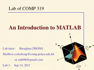
Lab 2 of COMP 319. Data and File in Matlab. Lab tutor : Shenghua ZHONG Email: zsh696@gmail.com csshzhong@comp.polyu.edu.hk Lab 2: Sep. 28, 2011. Outline of Lab 2. Review of Lab 1 Matlab vectors and arrays Matlab file (.m) building and saving

Lab 2 of COMP 319
E N D
Presentation Transcript
Lab 2 of COMP 319 Data and File in Matlab Lab tutor : Shenghua ZHONG Email: zsh696@gmail.com csshzhong@comp.polyu.edu.hk Lab 2: Sep. 28, 2011
Outline of Lab 2 • Review of Lab 1 • Matlab vectors and arrays • Matlab file (.m) building and saving • User defined function (if time is enough)
Outline of Lab 2 • Review of Lab 1 • (The path of Matlab:Y:\Win32\Matlab\R2011a) • 2. Matlab vectors and arrays • 3. Matlab file (.m) building and saving • 4. User defined function
Matlab Desktop Launch Pad Workspace Command Window Current Directory History
Matlab Help • Different ways to find information • help • help general, help mean, sqrt... • helpdesk - an html document with linksto further information
MATLAB Matrices • MATLAB treats all variables as matrices. For our purposes a matrix can be thought of as an array, in fact, that is how it is stored. • Vectors are special forms of matrices and contain only one row OR one column. • Scalars (標量)are matrices with only one row AND one column
Extracting a Sub-Matrix • A portion of a matrix can be extracted and stored in a smaller matrix by specifying the names of both matrices, the rows and columns. The syntax is: sub_matrix = matrix ( r1 : r2 , c1 : c2 ) ; where r1 and r2 specify the beginning and ending rows and c1 and c2 specify the beginning and ending columns to be extracted to make the new matrix.
Matlab Graphics x = 0:pi/100:2*pi; y = sin(x); plot(x,y) xlabel('x = 0:2\pi') ylabel('Sine of x') title('Plot of the Sine Function')
Outline of Lab 2 • Review of Lab 1 • Matlab vectors and arrays • Matlab file (.m) building and saving • User defined function
Vectors and Arrays in MATLAB • Matrix is the basic data structure of MATLAB • Vectors are special forms of matrices which contain only one row OR one column. • Array is another name of Matrix
Objectives of Introduction • This lab will discuss the basic calculations in the form of vectors and arrays. • For each of these collections, you will learn how to : • Create them • Manipulate them • Access their elements • Perform mathematical and logical operations on them
Vectors in Matlab • A vector is the simplest means of grouping a collection of same data items. • Vector elements have two separate and distinct attributes that make them unique in a specific vector: their numerical value and their position in that vector. • For example, the number 66 is in the third position in the vector. Its value is 66 and its index is 3. • There may be other items in the vector with the value of 66, but no other item will be located in this vector at position 3. Value: Index: 1 2 3 4 5 n-1 n
Create a Vector • There are two ways to create vectors that are directly analogous to the techniques for creating individual data items. • Creating vectors as a series of constant values • Producing new vectors by operating on existing vectors
Create Vectors of Constant Values • Enter the values directly In the command window, enter the following: >> A = [2, 5, 7, 1, 3] A = 2 5 7 1 3
Create Vectors of Constant Values • Enter the values as a range of numbers using the colon operator. The first number is the starting value, the second number is the increment, and the third number is the ending value. In the command window, enter the following: >> B = 1:3:20 B = 1 4 7 10 13 16 19
Create Vectors of Constant Values • Using the linspace() function to create a fixed number of values between two limits. The first parameter is the lower limit, the second parameter is the upper limit, and the third parameter is the number of values in the vector. First step: Help linspace; LINSPACE(X1, X2, N) generates N points between X1 and X2. Second step: write the function by yourself In the command window, enter the following: >> C = linspace(0, 20, 11) C = 0 2 4 6 8 10 12 14 16 18 20
Create Vectors of Constant Values • Using the functions zeros(1,n), ones(1,n), rand(1,n) (random numbers with uniform distribution), and rand(1,n) (random numbers with normal distribution) to create vectors filled with 0, 1, or random values between 0 and 1. In the command window, enter the following: >> E = zeros(1, 4) E = 0 0 0 0 >> F = ones(1, 4) E = 1 1 1 1 Do it yourselfabout how to use rand function
Contents in Workspace Window • The workspace window gives you several pieces of information about each of the variables/vectors you created: name, value, size, bytes, class, min, and max. • Notice that if the size of the vector is small enough, the value field shows its actual contents; otherwise, you see a description of its attributes, like <1 * 11 double>.
Index A Vector • As mentioned before, each element in a vector has two attributes: its value and its position in the vector. • You can access the elements in a vector in either of two ways: by indexing with a numerical vector or indexing with a logical vector.
Numerical Indexing • The elements of a vector can be accessed individually or in groups by enclosing the index of the one or more required elements in parentheses. Do it yourself (A = [2, 5, 7, 1, 3]) Change elements of a vector using the former exercise: >> A = [2, 5, 7, 1, 3]; >> A(5) = 42 A = 2 5 7 1 42
Numerical Indexing • A unique feature of Matlab is its behavior when attempting to write beyond the bound of a vector. Matlab will automatically extend the vector if you write beyond its current end. Do it yourself(A = [2, 5, 7, 1, 42]) Extend a vector using the former exercise: >> A = [2, 5, 7, 1, 42]; >> A(8) = 3 A = 2 5 7 1 42 0 0 3 • Note: Matlab extended the length to 8 and stored the value 0 in the unassigned elements.
Logical Indexing • So far, the only type of data we have used has been numerical values of type double. The logical operation is a different type of data, with values either true or false. Like numbers, logical values can be assembled into arrays by specifying true or false values. Below is an example, we can specify the variable mask as follows: >> mask = [true, false, false, true] mask = 1 0 0 1 • Note: the command window echoes the values of logical variables as if 1 represented true and 0 represented false.
Logical Indexing • We can index any vector with a logical vector as follows: >> mask = [true, false, false, true]; >> A = [2, 4, 6, 8, 10]; >> A(mask) ans = 2 8 • Note 1: When indexing with a logical vector the result will contain the elements of the original vector corresponding in position to the true values in the logical index vector. • Note 2: The logical index vector can be shorter than the source vector, but it cannot be longer.
Operating on Vectors • The essential core of the Matlab language is a rich collection of tools for manipulating vectors and arrays. First we show how these tools operate on vectors, and then generalizes to how they apply to arrays. • Arithmetic operations • Logical operations • Applying library functions • Concatenation • Slicing (generalized indexing)
Arithmetic Operations • Arithmetic operations can be performed collectively on the individual components of two vectors as long as both vectors are the same length, or one vector is a scalar. • Addition + a + b • Subtraction - a - b • Multiplication * or.* a*b or a.*b • Division / or ./ a/b or a./b
Arithmetic Operations Do it yourself In the command window, enter the following: >> A = [2, 5, 7, 1, 3]; >> A + 5 ans = 7 10 12 6 8 >> A*2 ans = 4 10 14 2 6
Arithmetic Operations Do it yourself (A = [2, 5, 7, 1, 3]) In the command window, enter the following: >> A = [2, 5, 7, 1, 3]; >> B = -1:1:3 B = -1 0 1 2 3 >> A .* B ans = -2 0 7 2 9 • Note: the sign .* means element-by-element multiplication.
Arithmetic Operations Do it yourself (A = [2, 5, 7, 1, 3]) In the command window, enter the following: >> A = [2, 5, 7, 1, 3]; >> B = -1:1:3 >> A * B ??? Error using ==> mtimes Inner matrix dimensions must agree. (the column size of A must be equal to the row size of B) >> C = [1, 2, 3]; >> A .* C ??? Error using ==> times Matrix dimensions must agree.
Exercise 1 • A is a row vector. The first element in A is 0, and the value vary from 0 to 10 with increment of 2 • B is row vector with six elements, and every variable in B is 2.5 • Calculate the value of C, which is equal to the sum of A and B • Calculate the value of D, which is equal to the element-by element multiplication between A and B • Change A(1,3) to 8. • Calculate E = A./B
Logical Operations • Logical operations can be performed element-by-element on two vectors as long as both vectors are the same length, or one vector is a scalar. The result will be a vector of logical values with the same length as the original vectors. Do it yourself >> A = [2, 5, 7, 1, 3]; >> B = [0, 6, 5, 3, 2]; >> A >= 5 ans = 0 1 1 0 0
Logical Operations Do it yourself (A = [2, 5, 7, 1, 3]; B = [0, 6, 5, 3, 2];) >> A = [2,5,7,1,3] >> A = [0,6,5,3,2] >> A >= B ans = 1 0 1 0 1 >> C = [1, 2, 3]; >> A > C ??? Error using ==> gt Matrix dimensions must agree.
Applying Library Functions • Matlab supplies the usual rich collection of mathematical functions that cover mathematical, and statistics capabilities. The following functions provide specific capabilities that are frequently useful: • sum(v) and mean(v) consume a vector and return the sum and mean of all the elements of the vector respectively. • min(v) and max(v) return two quantities: the minimum or maximum value in a vector, as well as the position in that vector where that value occurred. >> [value, where] = max([2, 7, 42, 9, -4]) value = 42 where = 3
Applying Library Functions • round(v),ceil(v), floor(v), and fix(v) remove the fractional part of the numbers in a vector by conventional rounding, rounding up, rounding down, and rounding toward zero, respectively. Do it yourself >> A = [1.1, 2.6, 3.7, -5.9, -6.4]; >> round(A) ans = 1 3 4 -6 -6 >> fix(A) ans = 1 2 3 -5 -6
Concatenation • Matlab lets us construct a new vector by concatenating other vectors, even an empty vector: A = [B C D … X Y Z] where the individual items in the brackets may be any vector. >> A = [2, 5, 7]; >> B = [1, 3]; >> [A B] ans = 2 5 7 1 3
Slicing (Generalized Indexing) >> A = [2, 5, 7, 1, 3, 4]; >> odds = 1:2:length(A); >> A(odds) ans = 2 7 3 • Line 1: create a vector A with 6 elements. • Line 2: define another vector odds. The function length() is used to refer to the size of a vector. • Line 3: Using vector odds to access elements in vector A. Since no assignment is made, the default variable ans takes on the value of a three-element vector containing the odd-numbered elements of A. Note: these are the odd-numbered elements, not the elements with odd values.
Exercise 2 • A=[1, 2.7, 8.9, -8, 4, 3.5] • B>0; • Return the sum and mean value of all the elements in A. • Return the max value of all elements in A. • fix(A)
Arrays in Matlab • Properties of an array • Create an array • Access and remove elements • Operating on arrays
Properties of An Array • A vector is the simplest way to group a collection of data items. This idea can be extended to arrays of multiple dimensions. • Our discussion will focus on two dimensional arrays. Properties and manipulations of arrays with higher dimensions are similar.
Properties of An Array • When a 2-D array has the same number of rows and columns, it is called square. • When the only nonzero values in a square occur when the row and column indices are the same, the array is called diagonal. • When there is only one row, the array is a row vector, or just a vector as you saw earlier. • When there is only one column, the array is a column vector, the transpose of a row vector.
Create An Array • Arrays can be created either by entering values directly, or by using built-in functions that create specific arrays. • Do it yourself • entering values directly. • >> A = [2, 5, 7; 1, 3, 42] • A = • 2 5 7 • 1 3 42
Create An Array Do it yourself >> z = zeros(2,3)>> rand(2,3) z =ans = 0 0 00.9501 0.6068 0.8913 0 0 00.2311 0.4860 0.7621 >> [z ones(2,4)] % concatenating arrays ans = 0 0 0 1 1 1 1 0 0 0 1 1 1 1
Access Elements of An Array • The elements of an array may be addressed by enclosing the indices of the required element in parentheses. The first index is the row index and the second index is the column index. Using the array A in the former example, • Do it yourself (A = [2, 5, 7; 1, 3, 42]) • >> A(2,3) >> A(2,3) = 0 • ans = A = • 42 2 5 7 • 1 3 0
Remove Elements From An Array (A = [2, 5, 7; 1, 3, 0]) >> A(:, 3)= [] A = 2 5 1 3 This command removes all elements from the third column in array A. >> A(2, :)= [] A = 2 5 This command removes all elements from the second row in array A.
Operating on Arrays • Operating on arrays is very similar to the operating on vectors. • Arithmetic operations • Logical operations • Applying library functions • Concatenation • Slicing (generalized indexing) • Reshaping arrays
Arithmetic Operations Do it yourself >> A = [2, 5, 7; 1, 3, 2]; >> A+5 ans = 7 10 12 6 8 7 >> B = ones(2, 3) B = 1 1 1 1 1 1 >> B = B * 2 B = 2 2 2 2 2 2
Logical Operations Do it yourself >> A = [2, 5; 1, 3]; >> B = [0, 6; 3, 2]; >> A > 4 ans = 0 1 0 0 >> A >= B ans = 1 0 0 1 >> C = [1, 2, 3, 4]; >> A > C ??? Error using ==> gt Matrix dimensions must agree.
Applying Library Functions • Below are some useful functions for array operation. • sum(v) or mean(v) when applied to a 2-D array return a row vector containing the sum or mean of each column of the array, respectively. If you want the sum of the whole array, use sum(sum(v)). • min(v) or max(v) return two row vectors: the minimum or maximum value in each column and also the row in that column where that value occurred. • max(max(y)) ormin(min(y)) return the minimum or maximum of the whole array. • >> [values rows] = max([2, 7, 42; 9, 14, 8; 10, 12, -6]) • values = 10 14 42 • rows = 3 2 1
Exercise 3 • A=[1, 2.7, 8.9, -8, 4, 3.5; 6.5, 8.9, 5, -0.9, 3, 19] ; • Set every element in six column to be 0.7. • Remove the second column in A; • Return the mean value of every column in A; • Return the mean value of whole A;
Concatenation Do it yourself >> A = [2, 5; 1, 7]; >> B = [1, 3]’; % transpose B and make a column vector >> [A B] ans = 2 5 1 1 7 3