
FILTERING
E N D
Presentation Transcript
FILTERING GG313 Lecture 27 December 1, 2005
A FILTER is a device or function that allows certain material to pass through it while not others. In electronics and signal analysis, a filter is a device or function that changes the shape of the phase and/or amplitude spectrum in the frequency domain, i.e. it attenuates energy at some frequencies relative to others, and it may also make considerable changes in phase, causing delays or advances in the time domain. A LINEAR TIME-INVARIENT (LTI) filter always behaves the same way regardless of the input or the time. For example a filter that attenuates 60 Hz energy by 48 dB, ALWAYS attenuates energy at 60 Hz by 48 dB. A LTI filter’s response is completely specified by its IMPULSE RESPONSE - the output when the input is an impulse.
A filter is CAUSAL if the output does not anticipate the input. A zero-phase filter (one that does not cause any delay) cannot be physically reliasable (except for a unit impulse). For example, consider a filter with the following impulse response: h=[.2 .2 .2 .2 .2] This filter is symmetric about its center (zero lag) and it will spread any signal at time t(i) over times t(i-2) to t(i+2). It thus sees AHEAD, and it can not be built with physical components. So it is noncausal. We can make this filter causal by adding zeros at the front, adding a 2-step delay: h=[0 0 .2 .2 .2 .2 .2] Now it spreads out the signal at t(i) from t(i) to t(i+4), and it does not see ahead.
Smoothing filters. Often you will have a power spectrum that is very noisy with large changes from one spectral estimate to another. In the case below it just looks like spikes. First, we take the log to see the “real” spectrum, and note that there is an underlying structure:
IF we want the underlying structure, we can convolve the power spectrum with a 25-point boxcar (each point =1/25) to obtain the heavy line below: and then exponentiate back to linear amplitude:
This type of boxcar filter is a moving average smoother. It is the same as taking a 25-point mean, moving one point, and taking another. Which domain you are in - time or frequency - is not important, smoothing filters work in both domains. Note that the transfer function of this smoothing filter is a sinc function - not a particularly good filter for separating signals with different frequencies. For that, we want a boxcar in the FREQUENCY domain, so the impulse response in the TIME domain will be a sinc function: This will be a low-pass filter, with infinite length, corner d.
Unless we want processing to take an infinite amount of time, we need to truncate the sinc function at some reasonable length in the time domain. What does truncation imply? - multiplying the impulse by a boxcar of some length. What does this do in the frequency domain? - convolves the boxcar with a sinc function:
The cost of truncating the sinc function in the time domain is some jitter in the “pass and stop bands”, and a less-steep slope between. The longer the sinc function kernel, the better. Note that this is a non-causal filter, but it is excellent for frequency separation. When is it important to use a causal filter? Consider the following seismogram: No trouble determining when the signal starts - an important feature of a good seismogram. What happens when we use it for input to a sinc filter:
The filtered seismogram looks fine, with a sharp onset, but look what happened to the start time: The red curve is the filtered one. Because the filter “sees” ahead of the signal, the start time is not correct.
What does a causal filter kernal look like? A causal low-pass filter, such as might result from an electronic filter, is an exponential: Causal R-C type low-pass filter impulse response Since this filter starts at zero time, it does not see ahead. The red curve is filtered with the causal filter. Note that the start time is preserved.
FIR Filters. The filters we have been discussing are all finite impulse response filters. These filters are defined by a kernel that is a fixed length time series that gets convolved with another time series to obtain a filtered output. Alternatively, the Fourier Transforms of the filter kernel can be multiplied by the Fourier Transform of the data series and inverse transformed to obtain the filtered signal. Let’s try one. GENERATE a random ~Gaussian time series by the following: y=(rand(1,512)-.5).*(rand(1,512)-.5).*(rand(1,512)-.5); subplot(1,2,1); plot(y) subplot(1,2,2); periodogram(y);
Generate a 7-point FIR smoothing filter and apply it. Also change subplot to “subplot( 2,2,-)” h=[1/7 1/7 1/7 1/7 1/7 1/7 1/7]; smoothing filter out=conv(y,h); convolution subplot(2,2,3); plot(out) subplot(2,2,4); periodogram(out); Run it
Generate a new filter by changing the MIDDLE value of h to a negative impulse equal in size to the sum of the other points: change all the subplot calls to subplot(3,2,-); hh=[1/7 1/7 1/7 -6/7 1/7 1/7 1/7]; outh=conv(y,hh); subplot(3,2,5); plot(outh); subplot(3,2,6); periodogram(outh); run it Edit the plots to get reasonable y axis limits.
There are many other ways to make high pass filters from low pass, but this one works, and it generates a high pass filter that has the same corner frequency as the low pass filter. IIR filters. Another type of filter has INFINITE IMPULSE RESPONSE, aslo called a RECURSIVE filter. It is designed using something called the z-transform, which we don’t have time to get into, and it is applied differently from a FIR filter. IIR filters are applied in a way more analogous to how filters are applied in the analog world than FIR filters. The earth cannot “convolve”.
Consider the function: This is not a simple convolution, because the output depends on previous OUTPUTS. Program this: n=128; x=zeros(1,n); x(1)=1; a0=1. b1=.5; out(1)=a0*x(1); for ii=2:n out(ii)=a0*x(ii)+b1*out(ii-1); end plot(out)
Notice that the input is an impulse. The output looks just like our causal filter from before, but we’re only doing 2 multiplications per output point, and the impulse resplonse goes on forever. What happens if the sign of b1 is negative? Note that a general IIR filter will be of the form: IIR filters are very fast relative to FIR filters, but they are somewhat noisier.