Download
1 / 30
300 likes | 582 Vues
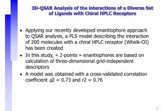
3D-QSAR Analysis of the interactions of a Diverse Set of Ligands with Chiral HPLC Receptors. Applying our recently developed enantiophore approach to QSAR analysis, a PLS model describing the interaction of 200 molecules with a chiral HPLC receptor (Whelk-OI) has been created

E N D
3D-QSAR Analysis of the interactions of a Diverse Set of Ligands with Chiral HPLC Receptors • Applying our recently developed enantiophore approach to QSAR analysis, a PLS model describing the interaction of 200 molecules with a chiral HPLC receptor (Whelk-OI) has been created • In this study, « 2-points » enantiophores are based on calculation of three-dimensional grid-independent descriptors • A model was obtained with a cross-validated correlation coefficient q2 = 0.73 and r2 = 0.76
Procedure 1) Compounds -> 2) Grid -> 3) Descriptors -> 4) Data Analysis Compound selection 1 Corina: Generation of 3D coordinates 3D structures 2 Grid calculations 3 Training data set 3) Transformation of interaction energies into receptor descriptors (binning) 4 Data analysis (PLS) Interaction energies Model Log(alpha)=a1 x S1 + a2 x S2 + a3 x S3 …..
Compound selection • 200 diverse molecules are extracted from ChirBase (alpha values vary from 1.00 to 13) • Structures are Converted to 3D by using Corina tool of the Tsar 3.3 software package and imported in Grid • Same analytical conditions (80:20 Hexane / 2-PrOH) • We tried to form a diverse data set 1) Compounds-> 2) Grid -> 3) Descriptors -> 4) Data Analysis
Choosing the Probes of the Grid Chiral Receptor amide Lipophile • Grid is generated by : • - Dry (Hydrophobic) • - O (carbonyl oxygen, H-bond acceptor) • - N (amide nitrogen, H-bond donor) 1) Compounds-> 2) Grid -> 3) Descriptors -> 4) Data Analysis
Grid Approach • Each molecule is positioned in a grid box. • The program Grid calculates the interaction energy of a probe atom with each molecule at points on a grid surrounding the molecules • Probes represent the potential receptor sites Grid Software is available from Molecular Discovery Ltd Probes: Acceptor Donor Hydrophobe (Lipophile) 0.3 A between grid points 1) Compounds-> 2) Grid -> 3) Descriptors -> 4) Data Analysis
Transformation of grid energies into descriptors coordinates of the grid points energies at grid point Grid • Compute the products of the energy values for all pairs of nodes within specified distance ranges (0.5, 1, 1.5, 2, 2.5 ….) • For each distance bin, we keep the highest product x y z -5 -2 -9 -5 -5 3 Molecule -0.001 -0.007 Probe Negative energies. correspond to favorable interactions 3 probes: L (Lipophile), D (H-donor), A (H-acceptor) Fast: few minutes / molecule Processing data grid 1) Compounds-> 2) Grid -> 3) Descriptors -> 4) Data Analysis
Transformation of grid energies into descriptors Acceptor - 2.3 kcal/mol 3Å D Donor 3Å - 5.8 kcal/mol A highest node-node binding is retained A 3Å - 3.5 kcal/mol D - 3.7 kcal/mol Couple of probes are selected in order to represent the best potential interactions with the receptor binding site (highest binding affinity). 1) Compounds-> 2) Grid -> 3) Descriptors -> 4) Data Analysis
Resulting Descriptor Data file Grid data are thus converted into inter-feature distances: AA: Acceptor-Acceptor DD: Donor – Donor LL: Lipophile – Lipophile AD: Acceptor – Donor AL Acceptor – Lipophile DL: Donor - lipophile 6 pairs of recognition sites (probes) X 20 distance ranges (0 to 10 A) = 120 descriptors for each molecule 0.5, 1, 1.5, 2, 2.5,3 … AA1, AA2, …AA20 DD1, DD2, …DD20 LL1, LL2,….LL20 AD1, AD2,….AD20 AL1, AL2, …AL20 DL1, DL2,….DL20 1) Compounds-> 2) Grid -> 3) Descriptors -> 4) Data Analysis
x2 y2 y1 PLS Approach • Plot data in K-Dimensional space - Orthogonal components Maximize the covariance x3 y3 Build new X Matrix T= XW weights Multivariate regression x1 Inputs Y=TQ+E Outputs X1,X2..Xn Y regression coefficients noise enantioselectivities Descriptors Y=XB+E (B=WQ) predictive regression model 1) Compounds-> 2) Grid -> 3) Descriptors -> 4) Data Analysis
PLS Results (6 components) • Performed using full cross-validation (leave one-out method: one entry is removed and model is rebuilt) • Model with the optimum number of PLS components (6), corresponding to the lowest predictive error sum of squares value was selected • Predictive ability of the model: Q2 = 0.73 • Correlation coefficient (Explained variance / Original variance): R2 = 0.76 It should be pointed that this model has been obtained across diverse data sources which originally contain a lot of noise 1) Compounds-> 2) Grid -> 3) Descriptors -> 4) Data Analysis
Predictions of the model 1) Compounds-> 2) Grid -> 3) Descriptors -> 4) Data Analysis
PLS factor contributions (regression coefficients ) Log(alpha)= a1 x AL1 + a2 x AL2 + a3 x AL3 ….. • Express the contribution of the descriptors to the model • PLS weights represent features important on receptor Short distance (2A) Distance increases Acceptor - lipophile Positive contributions Negative contributions 1) Compounds-> 2) Grid -> 3) Descriptors -> 4) Data Analysis
Putative favorable sites on receptor Lipophile Lipophile Acceptor Short distance 1) Compounds-> 2) Grid -> 3) Descriptors -> 4) Data Analysis
PLS factor contributions (regression coefficients ) Donor - lipophile 9 A 4 A 3 A 1) Compounds-> 2) Grid -> 3) Descriptors -> 4) Data Analysis
Putative favorable sites on receptor Lipophile Donor Lipophile 1) Compounds-> 2) Grid -> 3) Descriptors -> 4) Data Analysis
PLS factor contributions (regression coefficients ) 7 A Lipophile - lipophile 3 A 5 A 1) Compounds-> 2) Grid -> 3) Descriptors -> 4) Data Analysis
Putative favorable sites on receptor Lipophile Lipophile Lipophile 1) Compounds-> 2) Grid -> 3) Descriptors -> 4) Data Analysis
Acceptor - Acceptor 3-3.5 A Donor - Donor Negative contributions 1) Compounds-> 2) Grid -> 3) Descriptors -> 4) Data Analysis
Sites on receptor 2 Acceptors 1 Donor 1) Compounds-> 2) Grid -> 3) Descriptors -> 4) Data Analysis
External prediction data set • 28 molecules • Analytical conditions (80:20 Hexane / 2-PrOH) as chosen for the data set model • Poor alpha predictions: 10 molecules • Excellent alpha predictions: 12 molecules • Rather good prediction : 6 molecules 1) Compounds-> 2) Grid -> 3) Descriptors -> 4) Data Analysis
Examples (prediction set) In a given group of similar compounds, the same tendency can be found between experimental and predicted values alpha experimental 1.23 1.29 1.47 2.18 Alpha predicted 1.22 1.24 1.38 1.60 1) Compounds-> 2) Grid -> 3) Descriptors -> 4) Data Analysis
Examples (prediction set) alpha experimental 1.08 1.13 1.30 Alpha predicted 1.00 1. 16 1.25 1) Compounds-> 2) Grid -> 3) Descriptors -> 4) Data Analysis
Examples (prediction set) Poor predictions: alpha exp: 1.69 alpha pred: 5.4 alpha exp: 1.04 alpha pred: 1.60 Remark: Compounds poorly predicted contains original chemical features not found in the molecules of the model 1) Compounds-> 2) Grid -> 3) Descriptors -> 4) Data Analysis
Prediction set with extreme alpha values (=1.00 or > 3.00)(mixture of analytical conditions) • 22 molecules with excellent separation (alpha value > 3) • Predictions: - 17 molecules with alpha > 2.00 - 5 molecules with alpha > 1.08 and alpha < 1.15 – contain original chemical features not included in the model • 31 unresolved molecules (alpha = 1.00) • Predictions: - 15 molecules with alpha = 1.00 or < 1.08 : - 15 molecules with alpha > 1.1 and alpha < 2.5: • Best prediction performance for molecules • providing high enantioselectivities 1) Compounds-> 2) Grid -> 3) Descriptors -> 4) Data Analysis
Some good predictions (data set with alpha = 1.00) 1) Compounds-> 2) Grid -> 3) Descriptors -> 4) Data Analysis
Some good predictions (data set with alpha > 3.00) 1) Compounds-> 2) Grid -> 3) Descriptors -> 4) Data Analysis
Some insights afforded by the model Log(alpha)=a1 x AA1 + a2 x AA2 + … b1 x AD1+ ….. • Applying PLS model contributions to molecules may help to explain difference of enantioselectivity alpha exp = 1.29 alpha pred = 1.24 alpha exp = 2.37 Alpha pred= 2.63 Molecule 1 Molecule 2 Comparison of individual PLS factor contributions 1) Compounds-> 2) Grid -> 3) Descriptors -> 4) Data Analysis
Individual PLS factor contributions Log(alpha)=a1 x AA1 + a2 x AA2 + … Molecule 2: Positive effect of Donor - Donor on molecule 2 at long distance 9.5-10 A Acceptor – Acceptor on receptor a2xAA2 Molecule 2 a2xAA2 Molecule1 1) Compounds-> 2) Grid -> 3) Descriptors -> 4) Data Analysis
Enantioselectivity contribution plot • Interaction points are color coded according to the enantioselectivity contribution as given by the PLS model • Blue regions increase enantioselectivities
Other applications of Molecular Interaction fields Property Predictions on a given receptor: Example: Chirobiotic R High enantioselectivity for amino acids Most negative interaction provided by Grid: NH3+ -20.4774 kcal/mol COO- -14.1688 kcal/mol For whelk receptor: NH3+ -10.0489 kcal/mol COO- -7.5354 kcal/mol