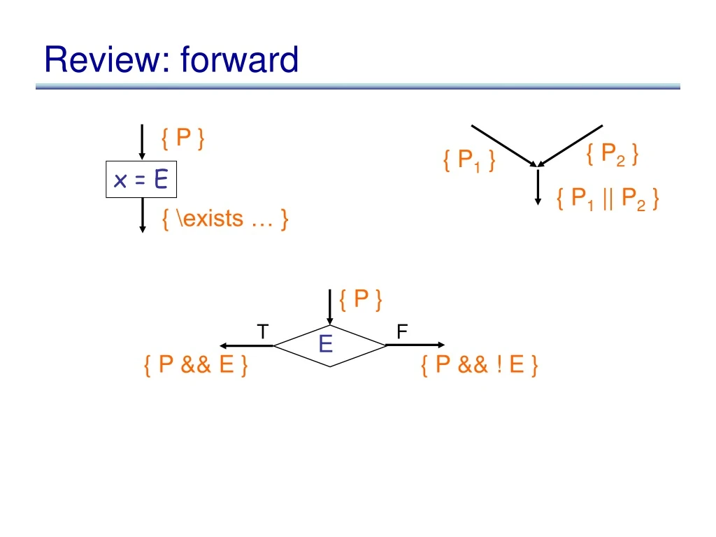
1. Review: forward { P } { P2 } { P1 } x = E { P1 || P2 } { \exists … } { P } T F E { P && E } { P && ! E }

2. Review: backward {Q[x:=E] } { P } { P } x = E { P } { Q } {(E ) P1) && (! E ) P2) } T F E { P1 } { P2 }

3. ESC Verification algorithm • Given function body annotated with pre-condition P and post-condition Q: • Compute wp of Q with respect to functon body • Ask a theorem prover to show that P implies the wp • We saw several examples last time • But we still haven’t seen how to handle: • loops, functions calls, and pointers

4. Reasoning About Programs with Loops • Loops can be handled using conditionals and joins • Consider the while(E) S statement { P } Loop invariant { I } { I } F T S E { Q } { I && E } if (1) P) I(loop invariant holds initially) and (2) I && ! E)Q(loop establishes the postcondition) and (3) { I && E } S { I }(loop invariant is preserved)

5. Loops in the backward direction • Given Q, want to find weakest invariant I that will establish (2) and (3), then pick P to be I • Finding weakest I is: • Undecidable in theory • Hard in practice { P } Loop invariant { I } { I } F T S E { Q } { I && E }

6. Loops in the forward direction • Given P, want to find strongest invariant I that will establish (1) and (3), then pick Q to be I && E • Again, finding I is hard { P } Loop invariant { I } { I } F T S E { Q } { I && E }

7. Loop Example • Let’s verify { x ==8 && y ==16 } while(x > 0) { x --; y -= 2; } { y==0 } • Is this true ? • We must find an appropriate invariant I • Try one that holds initially x == 8 && y == 16 • Try one that holds at the end y == 0 { x == 8 && y == 16 } { I } { I } x --; y -= 2 F T x > 0 { y == 0 } { I && x > 0 }

8. Loop Example (II) • Guess the invariant y == 2*x • Must check • Initial: x == 8 && y == 16 ) y == 2*x • Preservation: y == 2*x && x > 0 ) y – 2 = 2*(x – 1) • Final: y == 2*x && x <= 0 ) y == 0 { x == 8 && y == 16 } { y == 2*x } { y == 2*x } x --; y -= 2 F T x > 0 { y == 0 } { y == 2*x && x > 0 }

9. Loop Example (III) • Guess the invariant y == 2*x && x >= 0 • Must check • Initial: x == 8 && y == 16 ) y == 2*x && x >= 0 • Preservation: y == 2*x && x >= 0 && x > 0 ) y – 2 = 2*(x – 1)&& x – 1 >= 0 • Final: y == 2*x && x >= 0 && x <= 0 ) y == 0 { x == 8 && y == 16 } { y == 2*x && x >= 0} { y == 2*x && x >= 0} x --; y -= 2 F T x > 0 { y == 0 } { y == 2*x && x >= 0 && x > 0 }

10. Functions • Consider a binary search function bsearch int bsearch(int a[], int p) { { sorted(a) } … { r == -1 || (r >= 0 && r < a.length && a[r] == p) } return res; } • The precondition and postconditon are the function specification • Also called a contract Precondition Postcondition

11. Function Calls • Consider a call to function F(int in) • With return variable out • With precondition Pre, postcondition Post • Rule for function call: { P } if P)Pre[in:=E] } y = F(E) { Q } and Post[out := y, in := E])Q

12. Function Call Example • Consider the call { sorted(array) } y = bsearch(array, 5) if( y != -1) { { array[ y ] == 5 } • Show Post[r := y, a := array, p := 5] ) array[y] == 5 • Need to know y != -1 ! • Show sorted[array] ) Pre[a := array]

13. Function Calls: backward • Consider a call to function F(int in) • With return variable out • With precondition Pre, postcondition Post y = F(E) { Q }

14. Function Calls: backward • Consider a call to function F(int in) • With return variable out • With precondition Pre, postcondition Post y = F(E) { Q }

15. Pointers and aliasing { ??? } x = *y + 1 { x == 5 }

16. Pointers and aliasing { *y == 4 } Regular rule worked in this case! x = *y + 1 { x == 5 }

17. Example where regular rule doesn’t work x = *y + 1

18. Example where regular rule doesn’t work { ??? } x = *y + 1 { x == *y + 1 }

19. Example where regular rule doesn’t work { y != &x Æ x == *y + 1 } x = *y + 1 { x == *y + 1 }

20. Pointer stores { ??? } *x = y + 1 { y == 5 }

21. Pointer stores { (x == &y ) y + 1 == 5) Æ (x != &y ) y == 5) } *x = y + 1 { y == 5 }

22. One solution • Perform case analysis based on all the possible alias relationships between the LHS of the assignment and part of the postcondition • Can use a static pointer analysis to prune some cases out • However, exponentially many cases in the pointer analysis, which leads to large formulas. • eg, how many cases here: *x = *y + a { *z == *v + b }

23. Another solution • Up until now the program state has been implicit. Let’s make the program state explicit... • A predicate is a function from program states to booleans. • So for wp(S, Q), we have: • Q() returns true if Q holds in  • wp(S, Q)() returns true if wp(S, Q) holds in 

24. New formulation of wp • Suppose step(S, ) returns the program state resuling from executing S starting in program state . • Then we can express wp as follows: wp(S, Q)() =

25. New formulation of wp • Suppose step(S, ) returns the program state resuling from executing S starting in program state . • Then we can express wp as follows: wp(S, Q)() = Q(step(S, ))

26. Example in Simplify syntax From previous slide: wp(S, Q)() = Q(step(S, )) *x = y + 1 { y == 5 } Q is: step(S, ) is: wp(S, Q) is:

27. Example in Simplify syntax From previous slide: wp(S, Q)() = Q(step(S, )) *x = y + 1 { y == 5 } Q is: (EQ (select s y) 5) step(S, ) is: (store s (select s x) (+ (select s y) 1)) wp(S, Q) is: (EQ (select (store s (select s x) (+ (select s y) 1)) y) 5)

28. ESC/Java summary • Very general verification framework • Based on pre- and post-conditions • Generate VC from code • Instead of modelling the semantics of the code inside the theorem prover • Loops and procedures require user annotations • But can try to infer these

29. Search techniques

30. The map Logics Techniques Main search strategy Cross-cutting aspects Classical Non- classical lecture 2, 3 later in quarter Today we start techniques Applications Rhodium ESC/Java lecture 4 Predicate abstraction lecture 5 PCC later in quarter

31. Techniques in more detail Techniques Main search strategy Cross-cutting aspects

32. Techniques in more detail Main search strategy Cross-cutting aspects

33. Techniques in more detail Main search strategy • Theorem proving is all about searching • Categorization based on the search domain: • interpretation domain • proof-system domain Proof-system search ( ` ) Interpretation search (² )

34. Techniques in more detail • Equality... • common predicate symbol • Quantifiers... • need good heuristics • Induction... • for proving properties of recursive structures • Decision procedures... • useful for decidable subsets of the logic Cross-cutting aspects Equality Induction Quantifiers Decision procedures

35. ` E I ² Q D Main search strategy Cross-cutting aspects Proof-system search ( ` ) Equality Induction Interpretation search (² ) Quantifiers Decision procedures Techniques in more detail

36. ` E I ² Q D Searching • At the core of theorem proving is a search problem • In this course, we will categorize the core search algorithms based on what they search over • proof domain: search in the proof space, to find a proof • semantic domain: search in the “interpretation” domain, to make sure that there is no way of making the formula false • Before we dive in, let’s go back to some basic logic

37. ` E I ² Q D Logics • Suppose we have some logic • for example, propositional logic • or first-order logic

38. ` E I ² Q D The two statements `  ² one formula set of formulas “entails, or models” “is provable from ” In all worlds where the formulas in  hold,  holds  is provable from assumptions  Semantic Syntactic

39. ` E I ² Q D Interpretations • Intuitively, an interpretation I represents the “world” in which you evaluate a formula • Provides the necessary information to evaluate formulas • The structure of I depends on the logic • Interpretations are also sometimes called models

40. ` E I ² Q D Interpretations in PROP • Given a formula A Æ B , what do we need to evaluate it? • We need to know the truth values of A and B • In general, we need to know the truth values of all propositional variables in the formula • Note that the logical connectives are built in, we don’t have to say what Æ means

41. ` E I ² Q D Interpretations in FOL • Given a formula: 8 x. P(f(x)) ) P(g(x)), what do we need to know to evaluate it? • We need to know how the function symbol f and predicate symbol P operate • In general, need to know how all function symbols and predicate symbols operate • Here again, logical connectives are built-in, so we don’t have to say how ) operates.

42. ` E I ² Q D More formally, for PROP • An interpretation I for propositional logic is a map (function) from variables to booleans • So, for a variable A, I (A) is the truth value of A

43. ` E I ² Q D More formally, for FOL • An interpretation for first-order logic is a quadruple (D, Var, Fun, Pred) • D is a set of objects in the world • Var is a map from variables to elements of D • So Var(x) is the object that variable x represents

44. ` E I ² Q D More formally, for FOL • Fun is a map from function symbols to math functions • Fun(f) is the math function that the name f represents • For example, in the interpretation of LEQ(Plus(4,5), 10), we could have • D is the set of integers • Fun(4) = 4 , Fun(5) = 5 , Fun(10) = 10 , Fun(Plus) = + • But, we could also have Fun(Plus) = - • If f is an n-ary function symbol, then Fun(f) has type D n! D

45. ` E I ² Q D More formally, for FOL • Pred is a map from predicate symbols to math functions • Pred(P) is the math function that the name P represents • For example, in the interpretation of LEQ(Plus(4,5), 10) • we could have Pred(LEQ) = <= • If P is an n-ary predicate, then Pred(P) has type D n! bool

46. ` E I ² Q D Putting interpretations to use • We write «¬I to denote what  evaluates to under interpretation I • In PROP • «A¬I = I (A) • «:¬ I = true iff «¬ I is not true • «1Æ2¬I = true iff «1¬I and «2¬I are true • «1Ç2¬I = true iff «1¬I or «2¬I is true • etc.

47. ` E I ² Q D In FOL • « x ¬I = Var(x), where I = (D, Var, Fun, Pred) • « f(t1, …, tn) ¬ I = Fun(f)(« t1¬I , …, « tn¬I ), where I = (D, Var, Fun, Pred) • « P(t1, …, tn) ¬ I = Pred(P)(« t1¬I , …, « tn¬I ), where I = (D, Var, Fun, Pred) • Rules for PROP logical connectives are the same

48. ` E I ² Q D Quantifiers • « 8 x .  ¬(D, Var, Fun, Pred)= true iff forall o 2 D« ¬(D, Var[x := o], Fun, Pred)= true • « 9 x .  ¬(D, Var, Fun, Pred)= true iff there is some o 2 D for which« ¬(D, Var[x := o], Fun, Pred)= true

49. ` E I ² Q D Semantic entailment • We write ² , where  = {1, …n }, if for all interpretations I : • (Forall i from 1 to n « i¬ I = true) implies «  ¬ I = true • For example • { A ) B, B ) C} ² A ) C • { } ² (8 x. (P(x) Æ Q(x))) , (8 x. P(x) Æ8 x. Q(x)) • We write ² if { } ² • we say that  is a theorem

50. ` E I ² Q D Search in the semantic domain • To check that ² , iterate over all interpretations I and make sure that «  ¬ I = true • For propositional logic, this amounts to building a truth table • expensive, but can do better, for example using DPLL • For first-order logic, there are infinitely many interpretations • but, by cleverly enumerating over Herbrand’s universe, we can get a semi-algorithm