Total Solar Irradiance: Comparison of the Last Three Solar Cycles

1. Total Solar Irradiance: Comparison of the Last Three Solar Cycles Claus Fröhlich Physikalisch-Meteorologisches Observatorium Davos World Radiation Center CH 7260 Davos Dorf „Solar Variability and Earth‘s Climates, Monte Porzio Catone, 27 June – 1. July 2005

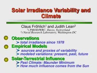
2. Outline • Introduction • Solar Irradiance Changes: Measurements • Total solar irradiance during the last 25 years • Solar Irradiance Changes: Mechanisms and Models • Sunspots and faculae • Network inside and outside active regions • Relation to solar surface magnetic fields • Solar Irradiance Changes:Reconstructions for the past • Proxies for solar activity: sunspot numbers, cosmogenic isotopes • Solar irradiance re-constructions • Conclusions „Solar Variability and Earth‘s Climates, Monte Porzio Catone, 27 June – 1. July 2005

3. Introduction (1 of 2) • Total solar irradiance (TSI) is the main power for the Earth-atmosphere system. Hence even small changes of TSI have the potential to change our climate. • 0.1% change of the solar constant yields a climate forcing of 1.365x0.7/4 = 0.24 Wm-2. This amount of forcing equals the forcing of recent 5-year increase of greenhouse gases – so it is small! • Due to the large inertia of the oceans changes on up to decadal scales – as e.g the solar cycle variation – are strongly attenuated, whereas changes on longer time-scales may well contribute global change if they exist. „Solar Variability and Earth‘s Climates, Monte Porzio Catone, 27 June – 1. July 2005

4. Introduction (2 of 2) For solar physics the challenge is to understand Maunder minimum type events and how magnetic fields influence irradiance. Solar activity is governed by magnetic fields which produce the dark sunspots, but also bright faculae.What is the role of the solar dynamo? „Solar Variability and Earth‘s Climates, Monte Porzio Catone, 27 June – 1. July 2005

5. TSI Database 1978 to present: What is available and which data contribute to the composite? • Since 1978 reliable TSI measurements from space are available from the following overlapping missions with electrically calibrated radiometers (ECR): • HF (Hickey-Frieden) on NIMBUS7 (17/11/1978 - 24/01/1993) • ACRIM-I on SMM (16/02/1980 - 01/06/1989) • ERBE on ERBS (24/10/1984 - 12/03/2003) • ACRIM-II on UARS (06/10/1991 - 27/09/2001) • SOVA on EURECA (11/08/1992 - 15/05/1993) • VIRGO (PMO6V, DIARAD) on SOHO (07/02/1996 - ………) • ACRIM-III on AcrimSat (05/04/2000 – ………) • TIM on SORCE (25/02/2003 - ………) • For the construction of the composite results from HF, ACRIM-I and II and VIRGO are used, with ACRIM-I as radiometric reference. • ERBE data are used as an independent dataset for comparison. As its sampling is so sparse (once every 14 days for a few minutes) daily data from a proxy model are also used for interpolation. „Solar Variability and Earth‘s Climates, Monte Porzio Catone, 27 June – 1. July 2005

6. TSI Database 1978 to present: What is available and which data contribute to the composite? • Note the differences in absolute scale: the 0.5% range at the beginning has been reduced to <0.2% for the ‘classical radiometers. However, the values from TIM on SORCE (in operation since February 2003) are about 4.8 Wm-2 (0.4%) lower (off scale). The reason for this large discre-pancy is not yet understood. • Only the ACRIMs, VIRGO and TIM radiometers have back-ups for in-flight determination of degradation. • The circled time-series are those used to construct the PMOD composite. „Solar Variability and Earth‘s Climates, Monte Porzio Catone, 27 June – 1. July 2005

7. TSI Database 1978 to present: What can be learned from VIRGO • The corrections for the changes of the radiometers in space are best illustrated with the measurements of the VIRGO experiment on SOHO • Level 1 data show quite different long-term behavior. Note the early increase of PMO6V radiometers. But also the completely different degradation behavior of PMO6V-A and DIARAD-L • Corrections for exposure-dependent changes are determined by comparison with less exposed radiometers (leading to level1.8). • By comparison of the time series of the two radiometer types possible exposure independent changes may be identified (leading to a combined level-2 data set) „Solar Variability and Earth‘s Climates, Monte Porzio Catone, 27 June – 1. July 2005

8. TSI Database 1978 to present: Corrections needed for the different TSI for the PMOD Composite • The HF and ACRIM data sets need corrections: • ACRIM-I data need a correction for the early increase and a change in the distribution of the degradation with time (both are calculated by applying the model developed for PMO6V) • HF data need to be corrected for glitches due to re-orientations of the S/C and other operational effects. As it has no spare there need to be corrections for early increase, degradation and a trend which may be exposure indepen-dent • ACRIM-II has some glitches and two of them are due to changes of the operational radiometer. „Solar Variability and Earth‘s Climates, Monte Porzio Catone, 27 June – 1. July 2005

9. TSI Database 1978 to present: Corrections needed for the different TSI for the PMOD Composite • First we repeat the illustra-tion of the corrections. • ACRIM-II is now shifted to the level of ACRIM-I by comparison with HF and ERBS • The HF and VIRGO data are shifted to the level of ACRIM-Iwhich is the radiometric reference. • Finally the composite is shifted to the level of SARR as defined by Crommelinck et al. (1995) „Solar Variability and Earth‘s Climates, Monte Porzio Catone, 27 June – 1. July 2005

10. TSI Database 1978 to present: Discussion of the PMOD, ACRIM and IRMB composites • A major result of the PMOD composite is that the Sun did not change during the last 25 years as manifested by the differ-ence between the minima of only 0.016 Wm-2. The peak-to-peak amplitudes decrease monotonically for the 3 cycles from 0.930 to 0.830 Wm-2 • The relative agreement with ACRIM-II and III and TIM confirms no trend The composite and VIRGO TSI can be fetched from: http://www.pmodwrc.ch/pmod.php?topic=tsi/composite/SolarConstant and http://www.pmodwrc.ch/pmod.php?topic=tsi/virgo/proj_space_virgo „Solar Variability and Earth‘s Climates, Monte Porzio Catone, 27 June – 1. July 2005

11. TSI Database 1978 to present: Discussion of the PMOD, ACRIM and IRMB composites • If the HF correction during the ACRIM gap is neglected, one gets the ACRIM composite. • The IRMB composite is a combination of all time series reduced to SARR and then added together. The ACRIM gap is bridged by comparison with ERBS. • Comparison of all composites with ERBS shows convincing evidence for the need of the HF corrections. The ERBS data in this plot have been corrected for the early increase with the coefficients determined for ACRIM-I and the dose of ERBS (total of 2.6 days of exposure) • The model is derived from magneto-grams by Wenzler et al. 2005. The ACRIM and IRMB composite can be fetched from: http://www.acrim.com/RESULTS/Composite/composite_nnaa3_hdr.res and http://remotesensing.oma.be/solarconstant/sarr/SARR.txt „Solar Variability and Earth‘s Climates, Monte Porzio Catone, 27 June – 1. July 2005

12. Estimation of the Uncertainty of the Composite TSI and of a Possible Trend • In order to asses the long-term uncertainty of the composite we may use the uncertainty of the slope of the comparison with ERBE which amounts to 4 ppm/a or 42 ppm over the time between the minima. Although this uncertainty is mainly due to the sampling noise in the ERBE data (Spearman rank =0.773) it may be used as an upper limit. The difference in slope of the ACRIM and PMOD composite is mainly due to the corrections of ACRIM-II not considered in the ACRIM composite. • The uncertainty of the HF corrections over the ACRIM gap is estimated to about 40ppm. • The trend determined by the difference of the two minima is –12ppm with a formal error of  5 ppm. The combined uncertainty of the corrections over the ACRIM gap (40 ppm) and those of ERBE comparison is about 60 ppm. Thus the trend is not significantly different from zero at the 5 level. • This uncertainty is astoundingly low compared to the estimated absolute uncertainty of the order of 1500 ppm. This is only possible with the overlapping measurements from two or more simultaneous missions. • Results from TIM on SORCE are lower by 0.35% than VIRGO or the SARR referred PMOD composite. It may indicate that the absolute uncertainty of the present radiometers used in space is underestimated or some effects exist which are not yet accounted for. „Solar Variability and Earth‘s Climates, Monte Porzio Catone, 27 June – 1. July 2005

13. Power Spectra of Irradiance Variability • The power spectrum of TSI includes periods up to the solar cycle from the PMOD composite and down to the 5-minute oscillations from the VIRGO data with a 1-minute sampling. The latter time series allows also compari-son of a quiet and active Sun. • The power spectra of the VIRGO/SPM (5nm wide spectral channels at 402, 500 and 861 nm) show how variable it is as a function of wavelength. • An interesting result is the ratio of active to quiet solar irradiance power. • From these power spectra the spectral re-distribution of power can also be deter-mined. „Solar Variability and Earth‘s Climates, Monte Porzio Catone, 27 June – 1. July 2005

14. Influence of Sunspots and Faculae • The series of images (July 1988) illustrates the darkening of sunspots and brightening by faculae • The two different effects are obvious from the histograms of the variance. The ratio of the two effects varies within and between the cycles. • From the position of the mode of the distribution the relative contributions of sunspots and faculae can be determined. „Solar Variability and Earth‘s Climates, Monte Porzio Catone, 27 June – 1. July 2005

15. Proxy Model of Irradiance Variations (1 of 2) • Sunspots can be modeled from their area and position on the disk by using an appropriate contrast. The result is the photometric sunspot index (PSI) • For faculae a similar approach could be applied. However, the areas are difficult to observe directly. So they have to be derived from plages, magnetograms or spot areas. Here, we use the MgII Index as a surro_-gate for faculae and net-work • The Mg index can easily be devided into short and long-term parts representing the faculae and network within and outside active regions. „Solar Variability and Earth‘s Climates, Monte Porzio Catone, 27 June – 1. July 2005

16. Proxy Model of Irradiance Variations (2 of 2) • The model is calibrated by regression of the three components PSI, MgIIst and MgIIlt with the PMOD composite. The resulting parameters are -1.158 ±0.007, 95.8±1.1, 117.8 ±0.7, respectively. The result can be improved by calibrating each cycle separately with changes of the parameters by up to 10% for PSI and MgIIst The model explains 73% of the variance. • Comparison with the mode results shows interesting differences which may be important for future improvement of the model. „Solar Variability and Earth‘s Climates, Monte Porzio Catone, 27 June – 1. July 2005

17. Reconstruction of Irradiance Variations in the Past (1 of 5) • The Zürich sunspot numbers were defined by Wolf and are in general used as representing the strength of the solar cycle • The cosmogenic isotopes vary in a similar way as the solar cycle amplitude of the sunspot number. This suggests that they might be used to infer the level of solar activity over even longer periods.They are produced by galactic cosmic rays which are modulated at Earth by the interplanetary magnetic field • The interplanetary magnetic field is determined by the open flux leaving the Sun and is monitored on Earth by e.g. the AA Index since 1868. The last data point in this plot is from July 2002. „Solar Variability and Earth‘s Climates, Monte Porzio Catone, 27 June – 1. July 2005

18. 1.7 Wm-2 Reconstruction of Irradiance Variations in the Past (2 of 5) • From MDI magnetogram one can determine the distribution of the magnetic field within an active region. From such distributions the facular pixels are selected according to 60G<B/<200G. Inside and outside active regions pixel with B/<60G are classified as network. Summing up the selected pixels and applying a corresponding -dependent contrast determined from the MDI continuum images (Ortiz et al. 2000) the facular and network contributions within an active region can be estimated • For averages over periods longer than the 27-day rotation the facular area is linearly correlated with the observed sunspot area in the same active region. Based on this correlation and with the -dependent contrast the facular brightening can be calculated. • Summing up the quiet sun pixels outside the active region and using the network contrast the solar minimum value can be determined and extrapolated to zero magnetic field (Foster, 2004) which yields a value of 1.7 Wm-2 below the present minima. „Solar Variability and Earth‘s Climates, Monte Porzio Catone, 27 June – 1. July 2005

19. Reconstruction of Irradiance Variations in the Past (3 of 5) • A problem surfaced with the quite different solar cycle 23 which shows no longer a very good correlation between sunspot numbers and irradiance • The short-term correlation seems to work, but the solar-cycle variations are no longer correlated to the degree observed for cycles 21 and 22. This influences the conclusion for both the solar-cycle and secular variations • One should certainly look for another proxy, maybe the aa index or for longer periods the production function  for 10Be and 14C. • Note that the the neutron monitor data are shifted by about 9 month for the odd cycles and the amplitude of the even cycle is higher. „Solar Variability and Earth‘s Climates, Monte Porzio Catone, 27 June – 1. July 2005

20. Q0 Q0 Reconstruction of Irradiance Variations in the Past (4 of 5) • Originally the picture from the Mount-Wilson Program showed convincing evidence of a Maunder-Minimum state of the Sun. • More recent data from the open cluster M67 and a detailed re-analysis of the Mount-Wilson data in terms of solar analogues does no longer support the bimodal distribution (Hall et al. 2004) • The Q0 value of a magneti-cally free Sun lies in the stellar units about 0.016 lower than the present solar minima. „Solar Variability and Earth‘s Climates, Monte Porzio Catone, 27 June – 1. July 2005

21. Reconstruction of Irradiance Variations in the Past (5 of 5) • The reconstruction of Foster (2004) is based on the fact that the Sun still had some magne-tism during the Maunder Minimum as manifested by the 10Be record. So, he lets the background contribution to go only half way down to Q0. • Comparison of the Foster reconstruction (blue) with trends Q0/2, with no trend (mauve) and with full trend to Q0.. The blue line is from the aa-index fitted to the composite. „Solar Variability and Earth‘s Climates, Monte Porzio Catone, 27 June – 1. July 2005

22. Conclusions • Solar irradiance varies with the 11-year solar cycle, being higher during solar maximum. At maxima TSI is higher by 0.930, 0.900 and 0.830 Wm-2 than the minima. • During the last 25 years of space measurements no trend can be inferred from our composite TSI. The observed difference between the minima of 0.016 Wm-2 is at the 5- level not different from zero. • The last 25 years of TSI can be satisfactorily modeled with 3 component proxy model describing the sunspot darkening and the brightening by faculae and network. • Reconstructions are based on the today’s understanding of the present Sun and the behaviour during the last 3 activity cycles – with the caveat that cycle 23 and somewhat lesser also 21 are different from cycle 22. • The present understanding postulates a TSI during e.g. the Maunder Minimum of only about 0.8 Wm-2 lower (3-4 times less than earlier estimates proposed). • The use of the sunspot number is somewhat questioned as a proxy for the decadal and century time variation of TSI. „Solar Variability and Earth‘s Climates, Monte Porzio Catone, 27 June – 1. July 2005

23. The End The presentation can be found on ftp://ftp.pmodwrc.ch/pub/claus/Rome2005/ CF_Rome_2005.ppt „Solar Variability and Earth‘s Climates, Monte Porzio Catone, 27 June – 1. July 2005

24. Introduction (2 of 3) • Although the ‚Solar Constant Program‘ of the Smithsonian Astrophysical Observatory was founded for the detection of solar irradiance changes and the possible influence on weather and climate operated for more than half a century, only modern satellite measurements were able to uniquely identify changes of TSI. • A possible connection between solar activity and climate and/or weather was speculated since the 11-year cycle of solar activity was detected by Schwabe. …….albeit with many failures. • The detection of TSI being higher during high activity brought new ideas about solar-climate connection mainly due to the coincidence of the ‚Little Ice Age‘ and the Maunder Minimum of solar activityin the 17th century (e.g. Eddy, 1976) „Solar Variability and Earth‘s Climates, Monte Porzio Catone, 27 June – 1. July 2005

25. Proxy Model of Irradiance Variations (4 of 4) • A 3-component model for TSI with PSI, short and long-term Mg index can explain 73% of the variance. A 2-component model with PSI and the Mg index yields a somewhat smaller correlation. • The sunspot component is well understood and PSI is quite reliable. Improvements could be incorporated by including a solar cycle dependent contrast, as suggested by photometric observations and the comparison with the mode. • It is interesting that the MgII Index works so well and that the long-term coefficient is about 1.5 times the short-term one.This is compatible with the fact, that it is due to the network (week magnetic elements in the magnetograms). Thus, the solar cycle variation is due to the network and not due to the active regions. „Solar Variability and Earth‘s Climates, Monte Porzio Catone, 27 June – 1. July 2005

26. Reconstruction of Irradiance Variations in the Past (2 of 6) Past irradiance variations are reconstructed according to the following schemes: • One method to reconstruct the 11-year solar cycle variation is based on the sunspot numbers calibrated in terms of irradiance by fitting the last three cycles to the composite. This provides a record back to the 16th century. Another method is using a model for facular brightening and the sunspot areas and locations of the Greenwich observations back to the late 19th century. • To add a secular change (background) by e.g. using the sunspot number envelope amplitude or the solar cycle length. The magnitude of the change between the Maunder Minimum and today is a free parameter and is determined by comparison with stellar analogues or from the irradiance of a magnetically free Sun. • Note that all the reconstructions are implicitly assuming that the Sun has the same features as observed during the last 25 years and – more importantly – that the secular changes are represented by sunspot numbers, which may be questioned „Solar Variability and Earth‘s Climates, Monte Porzio Catone, 27 June – 1. July 2005

27. Proxy Model of Irradiance Variations (3 of 3) • Another way to judge the correlation is from the results of bi-variate spectral analysis. • On average the correlation of 0.86 is confirmed. However, much lower correla-tions are found at various periods, among others around 500 days and at the 27-day solar rotation period. „Solar Variability and Earth‘s Climates, Monte Porzio Catone, 27 June – 1. July 2005