Exploring Dynamic Programming: Algorithms, Applications, and the Knapsack Problem
This chapter delves into dynamic programming as a key algorithmic paradigm for solving complex problems by breaking them down into overlapping sub-problems. It contrasts dynamic programming with greedy algorithms and divide-and-conquer strategies. The chapter highlights applications across various fields such as bioinformatics, control theory, and operations research. It also introduces famous algorithms like Bellman-Ford and the Knapsack Problem, illustrating the concepts through detailed examples and bottom-up approaches. The exposition emphasizes the importance of optimal substructure and the efficiency of dynamic programming.

Exploring Dynamic Programming: Algorithms, Applications, and the Knapsack Problem
E N D
Presentation Transcript
Algorithmic Paradigms • Greedy. Build up a solution incrementally, optimizing some local criterion. • Divide-and-conquer. Break up a problem into sub-problems, solve each sub-problem independently, and combine solution to sub-problems to form solution to original problem. • Dynamic programming.Break up a problem into a series of overlapping sub-problems, and build up solutions to larger and larger sub-problems.
Dynamic Programming Applications • Areas. • Bioinformatics. • Control theory. • Information theory. • Operations research. • Computer science: theory, graphics, AI, compilers, systems, …. • Some famous dynamic programming algorithms. • Linux diff for comparing two files. • Smith-Waterman for genetic sequence alignment. • Bellman-Ford for shortest path routing in networks. • Cocke-Kasami-Younger for parsing context free grammars.
Knapsack Problem • Knapsack problem. • Given n objects and a "knapsack." • Item i weighs wi > 0 kilograms and has value vi > 0. • Knapsack has capacity of W kilograms. • Goal: fill knapsack so as to maximize total value. • Ex: { 3, 4 } has value 40. • Greedy: repeatedly add item with maximum ratio vi / wi. • Ex: { 5, 2, 1 } achieves only value = 35 greedy not optimal. # value weight 1 1 1 2 6 2 W = 11 3 18 5 4 22 6 5 28 7
Dynamic Programming: False Start • Def. OPT(i) = max profit subset of items 1, …, i. • Case 1: OPT does not select item i. • OPT selects best of { 1, 2, …, i-1 } • Case 2: OPT selects item i. • accepting item i does not immediately imply that we will have to reject other items • without knowing what other items were selected before i,we don't even know if we have enough room for i • Conclusion. Need more sub-problems!
Dynamic Programming: Adding a New Variable • Def. OPT(i, w) = max profit subset of items 1, …, i with weight limit w. • Case 1: OPT does not select item i. • OPT selects best of { 1, 2, …, i-1 } using weight limit w • Case 2: OPT selects item i. • new weight limit = w – wi • OPT selects best of { 1, 2, …, i–1 } using this new weight limit
Knapsack Problem: Bottom-Up • Knapsack. Fill up an n-by-W array. Input: n, W, w1,…,wN, v1,…,vN for w = 0 to W M[0, w] = 0 for i = 1 to n for w = 1 to W if (wi > w) M[i, w] = M[i-1, w] else M[i, w] = max {M[i-1, w], vi + M[i-1, w-wi ]} return M[n, W]
0 1 2 3 4 5 6 7 8 9 10 11 0 0 0 0 0 0 0 0 0 0 0 0 { 1 } 0 1 1 1 1 1 1 1 1 1 1 1 { 1, 2 } 0 1 6 7 7 7 7 7 7 7 7 7 { 1, 2, 3 } 0 1 6 7 7 18 19 24 25 25 25 25 { 1, 2, 3, 4 } 0 1 6 7 7 18 22 24 28 29 29 40 { 1, 2, 3, 4, 5 } 0 1 6 7 7 18 22 28 29 34 34 40 Item Value Weight 1 1 1 2 6 2 3 18 5 4 22 6 5 28 7 Knapsack Algorithm W + 1 n + 1 OPT: { 4, 3 } value = 22 + 18 = 40 W = 11
Knapsack Problem: Running Time • Running time. (n W). • Not polynomial in input size! • "Pseudo-polynomial." • Decision version of Knapsack is NP-complete. [Chapter 8] • Knapsack approximation algorithm. There exists a poly-time algorithm that produces a feasible solution that has value within 0.01% of optimum. [Section 11.8]
String Similarity • How similar are two strings? • ocurrance • occurrence o c u r r a n c e - o c c u r r e n c e 6 mismatches, 1 gap o c - u r r a n c e o c c u r r e n c e 1 mismatch, 1 gap o c - u r r - a n c e o c c u r r e - n c e 0 mismatches, 3 gaps
Edit Distance • Applications. • Basis for Linux diff. • Speech recognition. • Computational biology. • Edit distance. [Levenshtein 1966, Needleman-Wunsch 1970] • Gap penalty ; mismatch penalty pq. • In general, 2 >= pq. • Cost = sum of gap and mismatch penalties. C T G A C C T A C C T - C T G A C C T A C C T C C T G A C T A C A T C C T G A C - T A C A T TC + GT + AG+ 2CA 2+ CA
Sequence Alignment • Goal: Given two strings X = x1 x2 . . . xm and Y = y1 y2 . . . yn of symbols, find alignment of minimum cost. • Def. An alignment M is a set of ordered pairs xi-yj such that each symbol occurs in at most one pair and no crossings. The number of xi and yj that don’t appear in M is the number of gaps. • Def. The pair xi-yj and xi'-yj'cross if i < i', but j > j'. • Ex:CTACCG vs. TACATG.Sol: M = x2-y1, x3-y2, x4-y3, x5-y4, x6-y6. x1 x2 x3 x4 x5 x6 C T A C C - G - T A C A T G y1 y2 y3 y4 y5 y6
Sequence Alignment: Problem Structure • Def. OPT(i, j) = min cost of aligning strings x1 x2 . . . xi and y1 y2 . . . yj. • Case 1: OPT matches xi-yj. • pay mismatch for xi-yj + min cost of aligning two stringsx1 x2 . . . xi-1 and y1 y2 . . . yj-1 • Case 2a: OPT leaves xi unmatched. • pay gap for xi and min cost of aligning x1 x2 . . . xi-1 and y1 y2 . . . yj • Case 2b: OPT leaves yj unmatched. • pay gap for yj and min cost of aligning x1 x2 . . . xi and y1 y2 . . . yj-1
Sequence Alignment: Algorithm • Analysis. (mn) time and space. • English words or sentences: m, n 10. • Computational biology: m = n = 100,000. • 10 billions ops OK, but 10GB array? Alignment(m, n, x1x2...xm, y1y2...yn, , ) { // A[0..m,0..n]: int array for i = 0 to m A[i, 0] = i for j = 1 to n A[0, j] = j for i = 1 to m A[i, j] = min([xi, yj] + A[i-1, j-1], + A[i-1, j], + A[i, j-1]) return A[m, n] }
Sequence Alignment: Algorithm Alignment(m, n, x1x2...xm, y1y2...yn, , ) { // A[0..m,0..n]: int array for i = 0 to m A[i, 0] = i for j = 1 to n A[0, j] = j for i = 1 to m A[i, j] = min([xi, yj] + A[i-1, j-1], + A[i-1, j], + A[i, j-1]) return A[m, n] } Assuming = 1 [xi, yj] = 0 if xi=yj [xi, yj] = 1 otherwise
Subequence Alignment • Goal: Given two strings X = x1 x2 . . . xm and Y = y1 y2 . . . yn of symbols, find alignment of X and a substring of Y with minimum cost. • Ex:CTACCG vs. TXYTACATGAH.Sol: Substring is TACATG and M = x2-y4, x3-y5, x4-y6, x5-y7, x6-y9.
Sequence Alignment: Problem Structure • Def. OPT(i, j) = min cost of aligning strings x1 x2 . . . xi and y1 y2 . . . yj. • Case 1: OPT matches xi-yj. • pay mismatch for xi-yj + min cost of aligning two stringsx1 x2 . . . xi-1 and y1 y2 . . . yj-1 • Case 2a: OPT leaves xi unmatched. • pay gap for xi and min cost of aligning x1 x2 . . . xi-1 and y1 y2 . . . yj • Case 2b: i < m and OPT leaves yj unmatched. • pay gap for yj and min cost of aligning x1 x2 . . . xi and y1 y2 . . . yj-1 • Case 2c: i == m and OPT leaves yj unmatched. • pay 0 for yj and min cost of aligning x1 x2 . . . xi and y1 y2 . . . yj-1
Subequence Alignment: Algorithm • Analysis. (mn) time and space. Alignment(m, n, x1x2...xm, y1y2...yn, , ) { // A[0..m,0..n]: int array for i = 0 to m A[i, 0] = i for j = 1 to n A[0, j] = 0 for i = 1 to m - 1 A[i, j] = min([xi, yj] + A[i-1, j-1], + A[i-1, j], + A[i, j-1]) A[m, j] = min([xm, yj] + A[m-1, j-1], + A[m-1, j], A[m, j-1]) return A[m, n] }
Longest common subsequence • The longest common subsequence (not substring) between “democrat” and “republican” is eca. • A common subsequence is defined by all the identical character • matches in an alignment of two strings. • To maximize the number of such matches, we must prevent substitution of non-identical characters, that is, 2 <= pq for p != q. • A[i, j] = min([xi, yj] + A[i-1, j-1], • + A[i-1, j], • + A[i, j-1])
Maximum Monotone Subsequence • A numerical sequence is monotonically increasing if the ith element is at least as big as the (i - 1)st element. • The maximum monotone subsequence problem seeks to delete the fewest number of elements from an input string S to leave a monotonically increasing subsequence. • Ex: A longest increasing subsequence of “243519698” is “24569.” • Let X be the input sequence and Y be the sorted input sequence. Then a longest increasing subsequence of X is also a longest common subsequence of X and Y, and vice versa. • Using the previous idea, we can solve this problem in O(n2) space and time. Can we do better?
Maximum Monotone Subsequence • A numerical sequence is monotonically increasing if the ith element is at least as big as the (i - 1)st element. Given X = x1 x2 . . . xn find the longest monotonically increasing subsequence of X. • Let OPT(i) be the longest monotonically increasing subsequence ending with xi. Then • OPT(1) = 1 and • OPT(i) = max(OPT(j)+1 : j < i and xj < xi ) MonotoneSubsequence(x1x2...xn) { // A[1..n]: int array for i = 1 to n { A[i] = 1 for j = 1 to i - 1 if (xi >= xj) A[i] = max(A[i], A[j]+1) } return max(A[1..n]) } // O(n) space, O(n2) time
Maximum Monotone Subsequence • MonotoneSubsequence returns the length of maximum monotone subsequence. How to return the maximum monotone subsequence? MonotoneSubsequence2(x1x2...xn) { y = MonotoneSubsequence(x1x2...xn) for k = 1 to n if (A[k] == y) i = k; S = []; while (i > 0) { S = xi + S for j = i – 1 to 1 if (xi >= xj && A[i] == A[j]+1) { i = j; break; } if (j < 1) break; } return S } // O(n) time