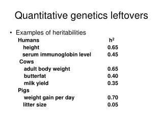
Chapter 9 Quantitative Genetics
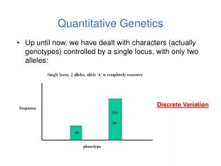
Chapter 9 Quantitative Genetics. Read Chapter 9. Traits such as cystic fibrosis or flower color in peas produce distinct phenotypes that are readily distinguished. Such discrete traits, which are determined by a single gene, are the minority in nature.

Chapter 9 Quantitative Genetics
E N D
Presentation Transcript
Chapter 9 Quantitative Genetics • Read Chapter 9. • Traits such as cystic fibrosis or flower color in peas produce distinct phenotypes that are readily distinguished. • Such discrete traits, which are determined by a single gene, are the minority in nature. • Most traits are determined by the effects of multiple genes.
Continuous variation • However, traits determined by many genes (polygenic traits) show continuousvariation. • Grain color in winter wheat is determined by three alleles at three loci.
Additive effects of genes • The genes affecting color of winter wheat interact in a particularly straightforward way. • They have additive genetic effects. • This means that the phenotype for an individual is obtained just by summing the effects of individual alleles. • The more alleles for dark color an individual has the darker it will be
Continuous variation • Examples in humans of traits that show continuous variation include height, intelligence, athletic ability, and skin color.
Quantitative traits • For continuous traits we cannot assign individuals to discrete categories. Instead we must measure them. • Therefore, characters with continuously distributed phenotypes are called quantitative traits.
Quantitative traits • Quantitative traits determined by influence of (1) genes and (2) environment.
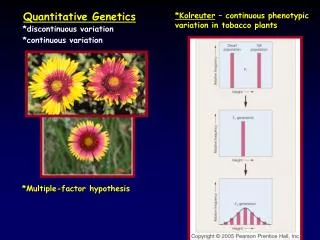
East (1916) • In early 20th century there was considerable debate over whether Mendelian genetics could explain continuous traits. • Edward East (1916) showed it could. • Studied longflower tobacco (Nicotianalongiflora)
East (1916) • East studied corolla length (part of flower) in tobacco flowers. • Crossed pure breeding short and long corolla individuals to produce F1 generation. Crossed F1’s to create F2 generation.
East (1916) • Using Mendelian genetics we can predict expected character distributions if character determined by one gene, two genes, or more etc.
East (1916) • Depending on number of genes: models predict different numbers of phenotypes. • One gene: 3 phenotypes • Two genes: 5 phenotypes • Six genes: 13 phenotypes. Continuous distribution.
East (1916) • How do we decide if a quantitative trait is under the control of many genes? • In one and two locus models many F2 plants have phenotypes like the parental strains. • Not so with 6-locus model. Just 1 in 4,096 individuals will have the genotype aabbccddeeff.
East (1916) • But, if Mendelian model works you should be able to recover the parental phenotypes through selective breeding. • East selectively bred for both short and long corollas. By generation 5 most plants had corolla lengths within the range of the original parents.
East (1916) • Plants in F5 generation of course were not exactly the same size as their ancestors even though they were genetically identical. • Why?
East (1916) • Environmental effects. • Depending on environment genetically identical organisms may differ greatly in phenotype.
Genetically identical plants grown at different elevations differ enormously (Clausen et al. 1948)
The importance of latent variation • Early work in the 2oth century on polygenic traits showed that new types or values of traits not seen in a parent population could appear in offspring produced by that population. • It was unclear where these new variants came from. It’s easy to see in figure A (next slide) how natural selection could favor some members of a population so that after a time the mean values of a population would increase within the range of previous variation.
The importance of latent variation • However, it’s less clear how a population could as a result of natural selection arrive at B in the previous slide in which the selected population is outside the range of the original population.
The key to understanding this phenomenon is to realize that when multiple genes contribute to a trait there will be many, many unique combinations of alleles that produce different phenotypes. • A population is not likely to include all of these possibilities. • Thus, a new variant can contain an assortment of alleles not seen previously. See next slide.
Gene interactions • Not all genes interact additively with the alleles’ effects summing together. • In many cases genes interact with each other nonadditively a phenomenon we call epistasis.
Gene interactions • For example, two loci influence coat color in oldfield mice, but they interact epistatically. • The effect of the Mc1R allele depends on which alleles are present at the agouti locus (next slide).
Population genetics of multiple loci • A locus is the physical location on a chromosome where a gene occurs. • Different versions of a gene are called alelles. • The Hardy-Weinberg models we have discussed so far are quite simple because they consider only a single locus and its alleles. • However, many traits are controlled by the combined influence of many genes.
Population genetics of multiple loci • Genes located on different chromosomes segregate (i.e. they enter gametes) independently of each other. • However, when genes are located on the same chromosome they frequently do not segregate independently, especially if they are located close to each other on a chromosome. Such loci have a physicallinkage.
Population genetics of multiple loci • The closer together two loci are on a chromosome the less likely it is that crossing over will occur between the loci during meiosis and split them up. • In most cases they will be inherited as a pair.
Population genetics of multiple loci • Consider a pair of loci located on same chromosome. • Gene at locus A has two alleles A and a • Gene at locus B has two alleles B and b
Population genetics of multiple loci • In two-locus Hardy-Weinberg analysis we track allele and chromosome frequencies. • Thus 4 possible chromosome genotypes are possible in previous slide: • AB, Ab, aB, ab • A multilocus genotype is referred to as a haplotype (from haploid genotype).
Statistical associations between loci • Does selection on locus A affect our ability to make predictions about evolution at locus B? • Sometimes. Depends on whether loci are in linkage equilibrium or linkage disequilibrium.
Statistical associations between loci • Two loci in a population are in linkageequilibrium when the genotype of a chromosome at one locus is independent of the genotype at the other locus on the same chromosome. • I.e. knowing genotype at one locus is of no use in predicting genotype at the other locus.
Statistical associations between loci • In contrast two loci are said to be in linkagedisequilibrium when knowing the allele at one locus enables you to predict what the allele at the other locus likely is. • For example in a population where there are AB, Ab, and aB haplotypes, but no ab haplotypes if we know an individual has a b allele we know that individual also has at least one A allele.
Quantifying linkage disequilibrium • To measure the associations between allele frequencies at two loci A and B we examine the haplotype frequencies at these loci. • Let fA, fB, fa and fb be the frequencies of the A, B, a and b alleles respectively. • Let hAB, hAb, haB, hab be the haplotype frequencies of AB, Ab, aB and ab haplotypes.
Quantifying linkage disequilibrium • If the allele at the A locus occurs independently of the allele at the B locus then the haplotype frequencies will be: • hAB = fAfB • hAb = fAfb • haB = fafB • hab = fafb
Quantifying linkage disequilibrium • So the expected haplotype frequency is found just by multiplying the appropriate allele frequencies by each other. • If the frequency of allele A (fA) = 0.7 and the frequency of allele B (fB) = 0.8 then the expected haplotype frequency hAB, if the alleles are in linkage equilibrium, would be 0.56.
Coefficient of linkage disequilibrium • To measure the degree of linkage disequilibrium we can calculate a coefficient of linkage disequilibroum (D). • For a given haplotype this is defined as the difference between the actual frequency we observe of a haplotype, e.g. AB, and the expected frequency fAfB of the same haplotype if the loci are independent. • D = hAB - fAfB
Coefficient of linkage disequilibrium • When the alleles at each locus occur independently then the coefficient of linkage disequilibrium will be zero. We then say the alleles are in linkage equilibrium. • If the alleles at each locus occur non-independently then the value of D will be non-zero and we say they are in linkage disequilibrium.
Coefficient of linkage disequilibrium • In a gene pool the frequencies of the alleles are as follows: A = 0.4, a= 0.6, B=0.3 and b= 0.7. • The haplotype frequencies are AB = 0.12, Ab =0.28, aB = 0.18 and ab=0.42. • Is the population in linkage equilibrium?
Coefficient of linkage disequilibrium • Yes. • hAB= 0.12 fAfB= 0.3*0.4 = 0.12 • hAb= 0.28 fAfb= 0.4*0.7 = 0.28 • haB= 0.18 fafB = 0.6*0.3 = 0.18 • hab= 0.42 fafb = 0.6*0.7 = 0.42 • For each haplotype D = zero e.g. D = hAB– fAfB= 0.12-0.12 = 0
Coefficient of linkage disequilibrium • In a second gene pool the frequencies of the alleles are as follows: A = 0.6, a= 0.4, B=0.8 and b= 0.2 • The observed haplotype frequencies are AB = 0.44, Ab =0.16, aB = 0.36 and ab=0.04. • Is this population in linkage equilibrium?
Coefficient of linkage disequilibrium • No. • hAB= 0.44 fAfB= 0.6*0.8 = 0.48 • hAb= 0.16 fAfb= 0.6*0.2 = 0.12 • haB= 0.36 fafB = 0.4*0.8 = 0.32 • hab= 0.04 fafb = 0.4*0.2 = 0.08 • For each haplotype D not equal to zero e.g. D = hAB– fAfB= 0.44-0.48 = -0.04
Coefficient of linkage disequilibrium • Another way to calculate the coefficient of linkage equilibrium if we just know haplotype frequencies is the following equation: • D = hABhab - hAbhaB • The value of this equation will be zero if the haplotypes are in linkage equilibrium.
Proof of the formula for linkage disequilibrium • D = hABhab - hAbhaB • Let p and q be the frequencies of alleles A and a. • Let s and t be the frequencies of alleles B and b. • If the population is in linkage equilibrium then • hAB = ps, hab = qt, hAb = pt, haB = qs • Therefore rewriting the equation for linkage disequilibrium in terms of allele frequencies we get • D = psqt - ptqs which equals zero if the population is in linkage equilibrium. • Any value of D not equal to zero implies the population is in linkage disequilibrium.
Coefficient of linkage disequilibrium • Is this population, which has the following haplotypes, in linkage equilibrium? • AB= 0.46, Ab = 0.14 aB = 0.34 ab= 0.06