Download
1 / 39
390 likes | 603 Vues
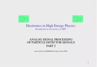
Electronics in High Energy Physics Introduction to electronics in HEP. Electrical Circuits (based on P.Farthoaut lecture at Cern). Electrical Circuits. Generators Thevenin / Norton representation Power Components Sinusoidal signal Laplace transform Impedance Transfer function

E N D
Electronics in High Energy PhysicsIntroduction to electronics in HEP Electrical Circuits (based on P.Farthoaut lecture at Cern)
Electrical Circuits • Generators • Thevenin / Norton representation • Power • Components • Sinusoidal signal • Laplace transform • Impedance • Transfer function • Bode diagram • RC-CR networks • Quadrupole
I r + v R - Sources • Voltage Generator • Current Generator
A A Rth Vth B B Thevenin theorem (1) • Any two-terminal network of resistors and sources is equivalent to a single resistor with a single voltage source • Vth = open-circuit voltage • Rth = Vth / Ishort
A A R1 + R1//R2 V R2 - Thevenin theorem (2) • Voltage divider
A A Rth Vth Rno Ino B B Norton representation • Any voltage source followed by an impedance can be represented by a current source with a resistor in parallel
I r + v R - Power transfer • Power in the load R • P is maximum for R = r
Complex notation • Signal : v1(t) = V cos( t + ) • v2(t) = V sin( t + ) • v(t) = v1 + j v2 = V e j( t + ) = V ej ej t = S ej t • Interest: • S = V ej contains only phase and amplitude • ej t contains time and frequency • Real signal = R [ S ej t ] • In case of several signals of same only complex amplitude are significant and one can forget ej t • One can separate phase and time
Complex impedance • In a linear network with v(t) and i(t), the instantaneous ratio v/i is often meaningless as it changes during a period • To i(t) and v(t) one can associate J ej t and S ej t • S / J is now independent of the time and characterizes the linear network • Z = S / J is the complex impedance of the network • Z = R + j X = z ej • R is the resistance, X the reactance • z is the module, is the phase • z, R and X are in Ohms • Examples of impedances: • Resistor Z = R • Capacitance (perfect) Z = -j / C; Phase = - /2 • 100 pF at 1MHz 1600 Ohms • 100 pF at 100 MHz 16 Ohms • Inductance (perfect) Z = jL; Phase = + /2 • 100 nH at 1 MHz 0.63 Ohms • 100 nH at 100 MHz 63 Ohms
Power in sinusoidal regime • i = IM cos t in an impedance Z = R + j X = z ej • v = z IM cos( t + ) = R IM cos t - X IM sin t • p = v i = R IM2 cos2t – X IM2 cost sin t = R IM2 /2 (1+cos2t ) - X IM2 /2 sin2 t • p = P (1+cos2 t ) - Pqsin2 t = pa + pq • pa is the active power (Watts); pa = P (1+ cos2t) • Mean value > 0; R IM2 /2 • pq is the reactive power (volt-ampere); pq = Pq sin2t • Mean value = 0 • Pq = X IM2 /2 • In an inductance X = L ; Pq > 0 : the inductance absorbs some reactive energy • In a capacitance X = -1/C; Pq < 0 : the capacitance gives some reactive energy
Cp Cs Rs Rp Real capacitance • A perfect capacitance does not absorb any active power • it exchanges reactive power with the source Pq = - IM2 /2C • In reality it does absorb an active power P • Loss coefficient • tg = |P/Pq| • Equivalent circuit • Resistor in series or in parallel • tg = RsCs • tg = 1/RpCp
Lp Ls Rs Rp Real inductance • Similarly a quality coefficient is defined • Q = Pq/P • Equivalent circuit • Resistor in series or in parallel • Q = Ls/Rs • Q = Rp/Lp
Laplace Transform (1) • v = f(i) integro-differential relations • In sinusoidal regime, one can use the complex notation and the complex impedance • V = Z I • Laplace transform allows to extend it to any kind of signals • Two important functions • Heaviside (t) • = 0 for t < 0 • = 1 for t 0 • Dirac impulsion (t) = ’(t) • = 0 for t 0
Laplace Transform (2) • Examples • Linearity • Derivation, Integration • Translation
Laplace Transform (3) • Change of time scale • Derivation, Integration of the Laplace transform • Initial and final value
I(p) i(t) Z(p) Z V(p) v(t) Impedances • Network v(t), I(t) • Generalisation • V(p) = Z(p) I(p)
I1 I2 TransferFunction V2 V1 Transfer Functions • Input V1, I1;Output V2, I2 • Voltage gain V2(p) / V1(p) • Current gain I1(p) / I2(p) • Transadmittance I2(p) / V1(p) • Transimpedance V2(p) / I1(p) • Transfer function Out(p) = F(p) In(p) • Convolution in time domain:
Bode diagram (1) • Replacing p with j in F(p), one obtains the imaginary form of the function transfer • F(j) = |F| ej() • Logarithmic unit: Decibel • In decibel the module |F| will be • The phase of each separate functions add • Functions to be studied
6 dB per octave 20 dB per decade a |F|dB [rad/s] 3 dB error Bode diagram (2) • F(p) = p + a ; |F1|db= 20 log | j + a| • Bode diagram = asymptotic diagram • < a, |F1| approximated with A = 20 log(a) • > a, |F1| approximated with A = 20 log() • 6 dB per octave (20 log2) or 20 dB per decade (20 log10) • Maximum error when = a • 20 log| j a + a| - 20 log(a) = 20 log (21/2) = 3 dB
[rad/s] -6 dB per octave |F|dB a - 20 dB per decade 3 dB error Bode diagram (3) • |F2|db= - 20 log | j + a| • Bode diagram = asymptotic diagram • < a, |F2| approximated with A = - 20 log(a) • > a, |F2| approximated with A = - 20 log() • - 6 dB per octave (20 log2) or - 20 dB per decade (20 log10) • Maximum error when = a • 20 log| j a + a| - 20 log(a) = 20 log (21/2) = 3 dB
[rad/s] |F|dB -20 dB per decade -40 dB per decade Bode diagram (4) • As before but: • Slope 6*n dB per octave (20*n dB per decade) • Error at =a is 3*n dB • Low pass filters
Bode diagram (5) • Phase of F1(j ) = (j + a) • tg = /a • Asymptotic diagram • = 0 when < a • = /4 when = a • = /2 when > a
Bode diagram (6) • Phase of F2(j ) = 1/(j + a) • tg =- /a • Asymptotic diagram • = 0 when < a • = - /4 when = a • = - /2 when > a
40 dB per decade b Bode diagram (7) • |F3|dB = 20 log|b2 - 2 + 2aj| • Asymptotic diagram • --> 0 A = 40 log b • --> ∞ A’ = 20 log 2 = 40 log • A = A’ for = b • Error depends on a and b • p2 + 2a p + b2 = b2[(p/b)2 + 2(a/b)(p/b) + 1] • Z = a/b U = /b
b -40 dB per decade Bode diagram (8) • |F4|dB = - 20 log|b2 - 2 + 2aj| • Asymptotic diagram • --> 0 A = - 40 log b • --> ∞ A’ = - 20 log 2 = - 40 log • A = A’ for = b • Error depends on a and b • Z = a/b U = /b
Z = 1 Z = 0.1 Bode diagram (9) • Phase of F3(j) = (b2 - 2 + 2aj) and F4(j) = 1/(b2 - 2 + 2aj) • tg = 2a/ (b2 - 2) • Asymptotic diagram • = 0 when < b • = ± /2 when = b • = ± when > b
V R Dirac response Heaviside response V2 V1 C t/RC RC-CR networks (1) • Integrator; RC = time constant
R V2 V1 C RC-CR networks (2) • Low pass filter • c = 1/RC
V Dirac response Heaviside response RC = 1 C R V1 V2 t/RC RC-CR networks (3) • Derivator; RC = time constant
Dirac response Heaviside response RiCi = RC V R2 C1 C2 V1 R1 V2 t/RC RC-CR networks (4)
R2 C1 C2 V1 R1 V2 RC-CR networks (5) • Band pass filter
y(t) = x(t) * f(t) Y(f) = X(f) F(f) f(t) F(f) x(t) X(f) Time or frequency analysis (1) • A signal x(t) has a spectral representation |X(f)|; X(f) = Fourier transform of x(t) • The transfer function of a circuit has also a Fourier transform F(f) • The transformation of a signal when applied to this circuit can be looked at in time or frequency domain
Time or frequency analysis (2) • The 2 types of analysis are useful • Simple example: Pulse signal (100 ns width) • (1) What happens when going through a R-C network? • Time analysis • (2) How can we avoid to distort it? • Frequency analysis
R Y(t) X(t) C Time or frequency analysis (3) • Time analysis
Time or frequency analysis (4) • Contains all frequencies • Most of the signal within 10 MHz • To avoid huge distortion the minimum bandwidth is 10-20 MHz • Used to define the optimum filter to increase signal-to-noise ratio
I1 I2 V1 V2 Quadrupole • Passive • Network of R, C and L • Active • Internal linked sources • Parameters • V1, V2, I1, I2 • Matrix representation
Parameters • Impedances • Admittances • Hybrids
Input and output impedances • Input impedance: as seen when output loaded • Zin = Z11 - (Z12 Z21 / (Z22 + Zu)) • Zin = h11 - (h12 h21 / (h22 + 1/Zu)) • Output impedance: as seen from output when input loaded with the output impedance of the previous stage • Zout = Z22 - (Z12 Z21 / (Z11 + Zg)) • 1/Zout = h22 - (h12 h21 / (h11+ Zg))