Download
1 / 42
420 likes | 497 Vues
Explore hypotheses explaining ozone trends, assess relevance to policy, and evaluate findings on changes in ambient ozone and precursor concentrations from 1990 to 2004 in Central California. Investigate reasons for varying ozone declines in different areas.

E N D
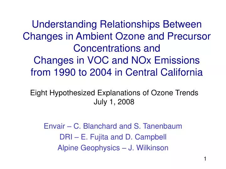
Understanding Relationships Between Changes in Ambient Ozone and Precursor Concentrations and Changes in VOC and NOx Emissions from 1990 to 2004 in Central California Eight Hypothesized Explanations of Ozone Trends July 1, 2008 Envair – C. Blanchard and S. Tanenbaum DRI – E. Fujita and D. Campbell Alpine Geophysics – J. Wilkinson
Today’s Topics • Identify hypotheses to explain ozone trends • Evaluate hypotheses • Discuss relevance to policy questions • Get feedback
Key Question • Substantial and statistically significant downward trends in NOx, NMOC, CO. • Generally downward trends in peak 8-hour ozone, but majority of sites less than 0.5 ppbv per year, only 7 of 42 statistically significant, and 10 sites have upward trends. • Why hasn’t peak ozone decreased as much in some areas as in others?
Hypothesis 1 • Ozone precursor emissions did not decline. Incorrect
1990 – 2004 AQ Trends Summary • No precursor trends significantly upward* • NOx sig* down at 22 of 28 sites** • CO sig* down at 21 of 25 sites** • NMOC sig* down at 6 of 7 sites*** *p < 0.05 ** At least 10 years data. One or both metrics: morning (5 – 11 am) or midday (time of peak 8-hour ozone). *** 7 - 10 years data, morning (5 – 8 am).
25 sites 7 sites 28 sites “7 x 7 Emissions” = in the 7x7 array of 4 km grid cells around a site
Hypothesis 2 • Ozone precursor emissions did not decline enough in some areas experiencing growth and development to produce a significant ozone response in those areas. Plausible
Boxes show where both NMOC and NOx emissions in the 7x7 arrays of 4 km grid cells (28 km x 28 km) surrounding monitoring sites decreased by less than 20 percent from 1990 to 2004
If local NMOC emissions unchanged, how much will ozone change?
Hypothesis 3 • Background* ozone concentrations increased. * Background ozone means ozone formed outside the North American boundary layer. Implausible
Mean peak 8-hour ozone in 1990-94 and in 2000-04 Ozone increases occurred at scattered sites in separate subregions
50 40 30 Lava Beds Mean Ozone (ppbv) Point Reyes Crater Lake 20 10 0 1994 1995 1996 1997 1998 1999 2000 2001 2002 2003 2004 2005 Year Lava Beds = -1011.904 + .528 * Year; R^2 = .438 Point Reyes = -1209.936 + .619 * Year; R^2 = .368 Crater Lake = -395.536 + .219 * Year; R^2 = .046 National Park Service Passive Ozone Monitoring Possible upward trend in background ozone of ~0.5 ppbv per year - if true, may make overall progress more difficult
Hypothesis 4 • Ozone trends were masked by changes in meteorological conditions. Implausible
Four meteorological types identified by PCA and K-means clustering
Year-to-year variations occurred in frequency of met types ….
…. But downward ozone trends did not depend upon met type ….
Hypothesis 5 Decreases in VOC emissions and reactivity slowed the rate of ozone formation but did not reduce the ultimate amount of ozone formed. Therefore, reductions of peak ozone occurred in urban cores and at near-downwind sites, but not at far downwind locations. Plausible
Measurements show ~30 – 120% decreases in ambient NMOC concentrations
Average reactivity* shows some declines (but mass decrease is larger and more important) *kOH weighted by mean annual concentrations (units are ppbC-1 sec-1)
Southern San Francisco Bay Area Southern San Francisco Bay Area 70000 70000 San Jose San Jose - - 4th 4th NMOC 1990 NMOC 1990 - - 1996 1996 60000 60000 NMOC 1997 NMOC 1997 - - 2004 2004 San Jose San Jose - - Piedmont Piedmont 50000 50000 Los Gatos Los Gatos 40000 40000 30000 30000 Fremont Fremont NMOC Emissions (tons/yr) NMOC Emissions (tons/yr) 20000 20000 Gilroy Gilroy 10000 10000 San Martin San Martin 0 0 0 0 20 20 40 40 60 60 80 80 100 100 Distance (km) Distance (km) In S Bay area, ozone declined at both urban and downwind sites
70000 70000 Sacramento and the Northern Sierra Foothills Sacramento and the Northern Sierra Foothills NMOC 1990 NMOC 1990 - - 1996 1996 60000 60000 Sac Sac - - Del Paso Del Paso NMOC 1997 NMOC 1997 - - 2004 2004 50000 50000 Sac Sac - - T St T St 40000 40000 Roseville Roseville 30000 30000 Folsom Folsom N. Highlands N. Highlands NMOC Emissions (tons/yr) NMOC Emissions (tons/yr) 20000 20000 10000 10000 Placerville Placerville Elk Grove Elk Grove Grass Valley Grass Valley Auburn Auburn 0 0 0 0 20 20 40 40 60 60 80 80 100 100 Distance (km) Distance (km) In Sacramento, ozone declines varied among sites.
70000 70000 Northern San Joaquin and Southern Sierra Foothills Northern San Joaquin and Southern Sierra Foothills 60000 60000 NMOC 1990 NMOC 1990 - - 1996 1996 NMOC 1997 NMOC 1997 - - 2004 2004 50000 50000 Modesto Modesto Turlock Turlock 40000 40000 30000 30000 NMOC Emissions (tons/yr) NMOC Emissions (tons/yr) Stockton Stockton - - Mariposa Mariposa Stockton Stockton - - Hazelton Hazelton 20000 20000 Merced Merced 10000 10000 San Andreas San Andreas Jackson Jackson Sonora Sonora Yosemite Yosemite - - Turtleback Turtleback 0 0 20 20 40 40 60 60 80 80 100 100 120 120 140 140 Distance (km) Distance (km) Ozone NMOC Emissions NMOC emissions did not decline in some parts of the N SJV and SSF. This makes it difficult to assess the argument that NMOC-control was not effective at the far downwind sites.
Hypothesis 6 Decreases in NOx emissions and concentrations resulted in less titration of ozone. Therefore, ozone concentrations increased in NOx-rich areas, but peak ozone declined in NOx-limited areas. Plausible
Ozone increases at night can be linked to lower NOx …. … But effects on peak ozone are difficult to interpret
90 80 70 Period 60 1990_1994 50 Ozone (ppbv) 1995_1999 40 2000_2004 30 20 Yosemite – Turtleback Dome 10 0 0 4 8 12 16 20 24 HOUR 90 80 70 Period 60 1990_1994 50 Ozone (ppbv) 1995_1999 40 2000_2004 30 20 Jerseydale 10 0 0 4 8 12 16 20 24 HOUR Mean Peak 8-Hour Ozone Mid-elevation Sierra Nevada sites show peak ozone improvements compared to early 1990s (but less change since the mid-1990s)
Hypothesis 7 • Greater or lesser decreases of VOC emissions compared to NOx emissions resulted in changes in VOC/NOx ratios, which led to changes in the efficiency of ozone production per unit of precursor mass. Plausible
Significance of VOC/NOx Ratios in Ozone Formation High VOC/NOx Termination Reaction at low VOC/NOx, removes NOx. Termination Reaction at high VOC/NOx, removes radicals. Low VOC/NOx Ozone formation is most efficient at VOC/NOx (ppbC/ppb) ratios between 10-12.
Morning (5 – 8 a.m.) NMOC/NOx ratios declined over time (Emission ratios average about 30% lower than ambient ratios)
Differences between morning and afternoon NMOC/NOx ratios declined
12 Noon – 2 p.m. 5 – 8 a.m Other ratios suggest changes in air mass ages or aging
Hypothesis 8 The validity of hypotheses 5, 6, and 7 varied during the trend period, with hypothesis 5 (VOC reductions ) having greater relevance early and hypotheses 6 (NOx reductions) and 7 (VOC/NOx ratios) increasing in importance toward the end. Plausible
Plausible Hypotheses H2: Emissions did not decline enough in some areas to affect ozone concentrations • Applicable in portions of N SJV & C SJV • NMOC emissions in affected area are ~20 percent of N & C SJV total
Plausible Hypotheses (continued) H5: VOC emission reductions were effective in urban centers and near-downwind areas but not far downwind • Ambient NMOC reductions are evident, but spatial patterns of ozone more complex than hypothesis • Difficult to infer causal link to ozone
Plausible Hypotheses (continued) H6: NOx emission reductions increased ozone in NOx-rich areas but reduced peak ozone at NOx-limited sites • Higher ozone during non-peak hours is probably related to decreased NO • Effects of NOx reductions on peak ozone are unclear
Plausible Hypotheses (continued) H7: Changes in VOC/NOx made ozone production more (or less) efficient • Declines in NMOC/NOx ratios occurred in measurements and the inventory • Differences between afternoon and morning NMOC/NOx ratios declined - may indicate that air mass ages and aging changed
Plausible Hypotheses (continued) H8: H5, H6, and H7 are all applicable, but differed in importance at different times • Consistent with data but difficult to demonstrate
Preliminary Implications • Observed ozone trends reflect emission changes and atmospheric chemistry • Ongoing emission reductions needed – including local reductions in some areas • NMOC emissions: some areas became more NMOC-sensitive. NMOC mass changes have probably been more important than reductions of reactivity