Operations Management Waiting-Line Models Module D
Operations Management Waiting-Line Models Module D. Outline. Characteristics of a Waiting-Line System. Arrival characteristics. Waiting-Line characteristics. Service facility characteristics. Waiting Line (Queuing) Models. M/M/1: One server. M/M/2: Two servers. M/M/S: S servers.


Operations Management Waiting-Line Models Module D
E N D
Presentation Transcript
Outline • Characteristics of a Waiting-Line System. • Arrival characteristics. • Waiting-Line characteristics. • Service facility characteristics. • Waiting Line (Queuing) Models. • M/M/1: One server. • M/M/2: Two servers. • M/M/S: S servers. • Cost comparisons.
Waiting Lines • First studied by A. K. Erlang in 1913. • Analyzed telephone facilities. • Body of knowledge called queuing theory. • Queue is another name for waiting line. • Decision problem: • Balance cost of providing good service with cost of customers waiting.
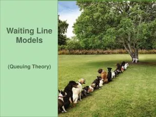
Thank you for holding. Hello...are you there? © 1995 Corel Corp. You’ve Been There Before! The average person spends 5 years waiting in line!! ‘The other line always moves faster.’
Waiting Line Examples Situation Arrivals Servers Service Process Bank Customers Teller Deposit etc. Doctor’s Patient Doctor Treatmentoffice Traffic Cars Traffic Controlledintersection Signal passage Assembly line Parts Workers Assembly
Waiting Line Components • Arrivals: Customers (people, machines, calls, etc.) that demand service. • Service System: Includes waiting line and servers. • Waiting Line (Queue): Arrivals waiting for a free server. • Servers: People or machines that provide service to the arrivals.
Key Tradeoff • Higher service level (more servers, faster servers) • Higher costs to provide service. • Lower cost for customers waiting in line (less waiting time).
Waiting Line Terminology • Queue: Waiting line. • Arrival: 1 person, machine, part, etc. that arrives and demands service. • Queue discipline: Rules for determining the order that arrivals receive service. • Channels: Parallel servers. • Phases: Sequential stages in service.
Input Characteristics • Input source (population) size. • Infinite: Number in service does not affect probability of a new arrival. • A very large population can be treated as infinite. • Finite: Number in service affects probability of a new arrival. • Example: Population = 10 aircraft that may need repair. • Arrival pattern. • Random: Use Poisson probability distribution. • Non-random:Appointments.
Number of events that occur in an interval of time. Example: Number of customers that arrive each half-hour. Discrete distribution with mean = Example: Mean arrival rate = 5/hour . Probability: Time between arrivals has a negative exponential distribution. Poisson Distribution
Poisson Probability Distribution Probability Probability =2 =4
Behavior of Arrivals • Patient. • Arrivals will wait in line for service. • Impatient. • Balk: Arrival leaves before entering line. • Arrival sees long line and decides to leave. • Renege: Arrival leaves after waiting in line a while.
Waiting Line Characteristics • Line length: • Limited: Maximum number waiting is limited. • Example: Limited space for waiting. • Unlimited: No limit on number waiting. • Queue discipline: • FIFO (FCFS): First in, First out.(First come, first served). • Random:Select next arrival to serve at random from those waiting. • Priority: Give some arrivals priority for service.
Service Configuration • Single channel, single phase. • One server, one phase of service. • Single channel, multi-phase. • One server, multiple phases in service. • Multi-channel, single phase. • Multiple servers, one phase of service. • Multi-channel, multi-phase. • Multiple servers, multiple phases of service.
Service system Served units Arrivals Queue Service facility Ship unloading system Ships at sea Empty ships Waiting ship line Dock Single Channel, Single Phase
Single Channel, Multi-Phase Service system Served units Arrivals Queue Service facility Service facility McDonald’s drive-through Cars in area Cars& food Waiting cars Pay Pick-up
Service system Served units Service facility Queue Arrivals Service facility Example: Bank customers wait in single line for one of several tellers. Multi-Channel, Single Phase
Service system Served units Service facility Service facility Queue Arrivals Service facility Service facility Example: At a laundromat, customers use one of several washers, then one of several dryers. Multi-Channel, Multi-Phase
Random: Use Negative exponential probability distribution. Mean servicerate = 6 customers/hr. Mean service time = 1/ 1/6 hour = 10 minutes. Non-random:May be constant. Example: Automated car wash. Service Times
Continuous distribution. Probability: Example: Time between arrivals. Mean servicerate = 6 customers/hr. Mean service time = 1/ 1/6 hour = 10 minutes =1 =2 =3 =4 Probability t>x Negative Exponential Distribution
Assumptions in the Basic Model • Customer population is homogeneous and infinite. • Queue capacity is infinite. • Customers are well behaved (no balking or reneging). • Arrivals are served FCFS (FIFO). • Poisson arrivals. • The time between arrivals follows a negative exponential distribution • Service times are described by the negative exponential distribution.
Steady State Assumptions • Mean arrival rate , mean service rate , and the number of servers are constant. • The service rate is greater than the arrival rate. • These conditions have existed for a long time.
Queuing Model Notation a/b/S • M = Negative exponential distribution (Poisson arrivals). • G = General distribution. • D = Deterministic (scheduled). Number of servers or channels. Service time distribution. Arrival time distribution.
Types of Queuing Models • Simple (M/M/1). • Example: Information booth at mall. • Multi-channel (M/M/S). • Example: Airline ticket counter. • Constant Service (M/D/1). • Example: Automated car wash. • Limited Population. • Example: Department with only 7 drills that may break down and require service.
Common Questions • Given , and S, how large is the queue (waiting line)? • Given and, how many servers (channels) are needed to keep the average wait within certain limits? • What is the total cost for servers and customer waiting time? • Given and, how many servers (channels) are needed to minimize the total cost?
Performance Measures • Average queue time = Wq • Average queue length = Lq • Average time in system = Ws • Average number in system = Ls • Probability of idle service facility = P0 • System utilization = • Probability of more than k units in system = Pn > k
= S 1 = = W L L L L W + + q s s s q q = = W W s q General Queuing Equations Given one of Ws ,Wq ,Ls,or Lq you can use these equations to find all the others.
M/M/1 Model • Type: Single server, single phase system. • Input source: Infinite; no balks, no reneging. • Queue: Unlimited; single line; FIFO (FCFS). • Arrival distribution: Poisson. • Service distribution: Negative exponential.
Average # of customers in system: L = s - 1 = Average time in system: W s - 2 Average # of customers in queue: L = q ( - ) Average time in queue: W = q ( - ) = M/M/1 Model Equations System utilization
- 1 M/M/1 Probability Equations Probability of 0 units in system, i.e., system idle: = - = P 1 0 Probability of more than k units in system: ( ) k+1 l = P n>k This is also probability of k+1 or more units in system.
M/M/1 Example 1 Average arrival rate is 10 per hour. Average service time is 5 minutes. = 10/hr and = 12/hr (1/ = 5 minutes = 1/12 hour) Q1: What is the average time between departures? 5 minutes? 6 minutes? Q2: What is the average wait in the system? 1 = W = 0.5 hour or 30 minutes s 12/hr-10/hr
1 1 1 1 = W W W + s q 2 12 q Also note: so O.41667 hours - = = W - = s M/M/1 Example 1 = 10/hr and = 12/hr Q3: What is the average wait in line? 10 O.41667 hours = 25 minutes = = W q 12 (12-10)
L L q s M/M/1 Example 1 = 10/hr and = 12/hr Q4: What is the average number of customers in line and in the system? 102 4.1667 customers = = L q 12 (12-10) 10 5 customers = = L s 12-10 Also note: = W = 10 0.41667 = 4.1667 q = W = 10 0.5 = 5 s
- 1 M/M/1 Example 1 = 10/hr and = 12/hr Q5: What is the fraction of time the system is empty (server is idle)? 10 = - = = = 16.67% of the time P 1 - 1 0 12 Q6: What is the fraction of time there are more than 5 customers in the system? ( ) 6 10 = 33.5% of the time = P n>5 12
More than 5 in the system... • Note that “more than 5 in the system” is the same as: • “more than 4 in line” • “5 or more in line” • “6 or more in the system”. All are P n>5
( ) 5 10 1 - P = 1 - 0.402 = 0.598 or 59.8% = 1 - n>4 12 M/M/1 Example 1 = 10/hr and = 12/hr Q7: How much time per day (8 hours) are there 6 or more customers in line? = 0.335 so 33.5% of time there are 6 or more in line. P n>5 0.335 x 480 min./day = 160.8 min. = ~2 hr 40 min. Q8: What fraction of time are there 3 or fewer customers in line?
M/M/1 Example 2 Five copy machines break down at UM St. Louis per eight hour day on average. The average service time for repair is one hour and 15 minutes. = 5/day ( = 0.625/hour) 1/ = 1.25 hours = 0.15625 days = 1 every 1.25 hours = 6.4/day Q1: What is the number of “customers” in the system? 5/day = 3.57 broken copiers = L S 6.4/day-5/day
M/M/1 Example 2 = 5/day (or = 0.625/hour) = 6.4/day (or = 0.8/hour) Q2: How long is the average wait in line? 5 W = 0.558 days (or 4.46 hours) = q 6.4(6.4 - 5) 0.625 W = 4.46 hours = q 0.8(0.8 - 0.625)
M/M/1 Example 2 = 5/day (or = 0.625/hour) = 6.4/day (or = 0.8/hour) Q3: How much time per day are there 2 or more broken copiers waiting for the repair person? 2 or more “in line” = more than 2 in the system ( ) 3 5 P = = 0.477 (47.7% of the time) n>2 6.4 0.477x 480 min./day = 229 min. = 3 hr 49 min.
M/M/S Model • Type: Multiple servers; single-phase. • Input source: Infinite; no balks, no reneging. • Queue: Unlimited; multiple lines; FIFO (FCFS). • Arrival distribution: Poisson. • Service distribution: Negative exponential.
M/M/S Equations Probability of zero people or units in the system: Average number of people or units in the system: Average time a unit spends in the system: Note: M = number of servers in these equations
M/M/S Equations Average number of people or units waiting for service: Average time a person or unit spends in the queue:
4 W = s 42 - 2 L L 2 s q W = q (2 + )(2 -) = = W W q s 2 - P = 0 2 + M/M/2 Model Equations Average time in system: Average time in queue: Average # of customers in queue: Average # of customers in system: Probability the system is empty:
M/M/2 Example Average arrival rate is 10 per hour. Average service time is 5 minutes for each of 2 servers. = 10/hr, = 12/hr, and S=2 Q1: What is the average wait in the system? 412 W = 0.1008 hours = 6.05 minutes = s 4(12)2 -(10)2
1 1 = W W W + q s q M/M/2 Example = 10/hr, = 12/hr, and S=2 Q2: What is the average wait in line? (10)2 W = 0.0175 hrs = 1.05 minutes = q 12 (212 + 10)(212 - 10) Also note: so 0.1008 - 0.0833 =0.0175 hrs = W - = s
L L q s M/M/2 Example = 10/hr, = 12/hr, and S=2 Q3: What is the average number of customers in line and in the system? = W = 10/hr 0.0175 hr = 0.175 customers q = W = 10/hr 0.1008 hr = 1.008 customers s
M/M/2 Example = 10/hr and = 12/hr Q4: What is the fraction of time the system is empty (server is idle)? 212 - 10 P = 41.2% of the time = 0 212 + 10
M/M/1, M/M/2 and M/M/3 1 server2 servers3 servers Wq 25 min. 1.05 min. 0.1333 min. (8 sec.) 0.417 hr 0.0175 hr 0.00222 hr WS 30 min. 6.05 min. 5.1333 min. Lq 4.167 cust. 0.175 cust. 0.0222 cust. LS 5 cust. 1.01 cust. 0.855 cust. P0 16.7% 41.2% 43.2%
Service Cost per Day = 10/hr and = 12/hr Suppose servers are paid $7/hr and work 8 hours/day and the marginal cost to serve each customer is $0.50. M/M/1 Service cost per day = $7/hr x 8 hr/day + $0.5/cust x 10 cust/hr x 8 hr/day = $96/day M/M/2 Service cost per day = 2 x $7/hr x 8hr/day + $0.5/cust x 10 cust/hr x 8 hr/day = $152/day