Compression techniques.
Compression techniques. Why we need compression. Types of compression Lossy and lossless Concentrate on lossless techniques. Run Length coding. Entropy or variable length coding. Huffman coding. DCT (Discrete Cosine Transform)

Compression techniques.
E N D
Presentation Transcript
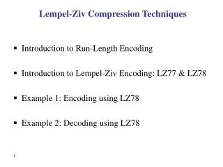
Compression techniques. • Why we need compression. • Types of compression • Lossy and lossless • Concentrate on lossless techniques. • Run Length coding. • Entropy or variable length coding. Huffman coding. • DCT (Discrete Cosine Transform) • Not a compression technique itself, but allows the introduction of other techniques.
Compression • Digitised sound and video produces a lot of data. • In particular digitised television quality pictures produce data at 270 Mbits/second which is faster than most hard disks, CD roms and networks devices can accommodate. • We need to compress data for use on computers.
Compression • We have two types of compression. • Lossy compression and lossless compression. • As the names suggest lossy compression loses some of the original signal, while lossless does not. • Lossless techniques such as run-length encoding and Huffman coding achieve compression by creating shorter codes. This is not always possible.
Compression • Lossy techniques rely on throwing away some information which the viewer or listener will not notice too much. • Involves changing the data to some other form. (Transform) • Most lossy techniques are noticeable. • The more lossy compression that is applied, the more the compression effect will be noticeable.
Probability. • Consider the throwing of a die. • What is the probability of, say of throwing a 5. • In this equal probability problem the probability of throwing any specified number between 1 and 6 is a sixth.
Probability. • Now make up a short sentence, for example. • “This is the best class that I have ever taught” • The sentence does not have to be true for the exercise. • Work out the probability of finding an ‘e’ in the sentence. The probability of finding any given letter is not equal in this example. • There are four e’s in the sentence which have a total of 37 letters the probability of finding an ‘e’ is then 4/37.
Information. • When we send pictures, sound and text we are sending information. • Information is closely related to probability. • For example, if the die had the same number on each side then we would know the answer of any “throw” without being given any information. • The lower the probability of a piece of data then the greater the information.
Entropy (variable length) coding (VLC) • The idea is to give shorter codes to values (symbols) which occur most frequently and longer codes to infrequently occurring values. • Therefore more information takes longer codes and less information is given shorter codes. • Huffman coding is an example of such a variable length code.
Huffman coding • The following algorithm generates Huffman code: • Find (or assume) the probability of each values occurrence. • Order the values in a row of a table according to their probability. • Take the two symbols with the lowest probability, and place them as leaves on a binary tree. • Form a new row in the table replacing the these two symbols symbols with a new symbol. This new symbol forms a branch node in the tree. Draw it in the tree with branches to its leaf (component) symbols • Assign the new symbol a probability equal to the sum of the component symbol’s probability.
Huffman coding • Repeat the above until there is only one symbol left. This is the root of the tree. • Nominally assign 1’s to the right hand branches and 0’s to the left hand branches at each node. • Read the code for each symbol from the root of the tree.
Huffman coding Examples • Form a Huffman code based upon the following symbols and associated probabilities (in brackets) A(0.5) B(0.15) C(0.15) D(0.1) E(0.1) Form Huffman tree: Take 2 symbols with lowest probability add as leaves to the tree (see next slide), and create new row combining these 2 symbols, with a probability equal to the sum of the 2 symbols probability: A(0.5) B(0.15) C(0.15) DE(0.2) Draw branch node DE on the tree connecting to D and E Continue repeat the above until one symbol left. A(0.5) BC(0.3) DE(0.2) A(0.5) BCDE(0.5) ABCDE(1) Try your own with the following symbols A(0.2) B(0.1) C(0.3) D(0.05) E(0.35)
Limits of Huffman coding (worst case) • When all the probabilities are equal. • That is there is no statistical bias. • Example • A(1/8), B(1/8), C(1/8), D(1/8) • E(1/8), F(1/8), G(1/8). H(1/8) Figures in brackets are probabilities Construct Huffman tree: • A(1/8), B(1/8), C(1/8), D(1/8) E(1/8), F(1/8), G(1/8). H(1/8) • AB(1/4), C(1/8), D(1/8) E(1/8), F(1/8), G(1/8). H(1/8) • AB(1/4), CD(1/4), E(1/8), F(1/8), G(1/8). H(1/8) • AB(1/4), CD(1/4), E(1/8), F(1/8), G(1/8). H(1/8) • AB(1/4), CD(1/4), EF(1/4), G(1/8), H(1/8) • AB(1/4), CD(1/4), EF(1/4), GH(1/4) • ABCD(1/2), EFGH(1/2) • ABCDEFGH(1)
Limits of Huffman coding (worst case) Reading the codes A 111 E 011 B 110 F 010 C 101 G 001 D 100 H 000
Limits of Huffman coding (best case) • When all the probabilities change in powers of 2. • That is there is optimum statistical bias. • Example • A(1/128), B(1/128), C(1/64), D(1/32) • E(1/16), F(1/8), G(1/4). H(1/2) Figures in brackets are probabilities Construct Huffman tree: • A(1/128), B(1/128), C(1/64), D(1/32), E(1/16), F(1/8), G(1/4). H(1/2) • AB(1/64), C(1/64), D(1/32), E(1/16), F(1/8), G(1/4). H(1/2) • ABC(1/32), D(1/32), E(1/16), F(1/8), G(1/4). H(1/2) • ABCD(1/16), E(1/16), F(1/8), G(1/4). H(1/2) • ABCDE(1/8), F(1/8), G(1/4). H(1/2) • ABCDEF(1/4), G(1/4). H(1/2) • ABCDEFG(1/2). H(1/2) • ABCDEFGH(1)
Limits of Huffman coding (best case) Reading the codes A 1111111 E 1110 B 1111110 F 110 C 111110 G 10 D 11110 H 0
Huffman coding Examples • Repeat the above until there is only one symbol left. This is the root of the tree. • Nominally assign 1’s to the right hand branches and 0’s to the left hand branches at each node. • Read the code for each symbol from the root of the tree.
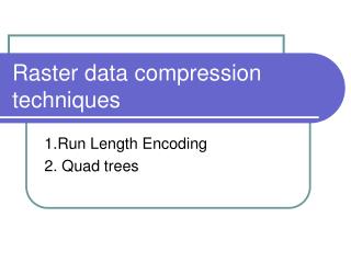
Run length coding • Another lossless technique. • Suppose we have a sequence of values: • S=1 2 2 2 1 1 3 3 3 3 3 1 1 6 6 6 6. • The sequence uses 17 separate values. • We could code this by saying: • We have one 1, three 2’s , 2 1’s …….. • In run length code this would be • 1 1 3 2 2 1 5 3 2 1 4 6 • Taking only 12 values • No use if we don’t have runs • 1 5 6 8 9 five values would be coded. • 1 1 1 5 1 6 1 8 1 9 taking ten values.
Run length coding • We also have to decide and specify how many spaces we will leave for the data and how much for the run length value. • For example, in the above the values and the run lengths are all less than 10, the spaces are inserted to explain the principle. • The code 113221532146 could mean 11 3’s, 22 1’s, 53 2’s and 14 6’s if we did not know the allocation of data for the values and the run length. • It will be inefficient to allocate this data without consideration of the original data.
Exercises • Calculate a Huffman code for your sentence above. Check what compression is achieved. • Express the following sequence as a run length code, specifying your data allocation. 1 1 1 12 1 23 54 54 56 3 111 111 111