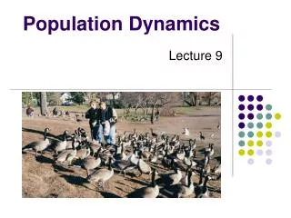
Population Dynamics
Population Dynamics . Population – a group of organisms of the same species occupying a particular space at a particular time. Demes – groups of interbreeding organisms local population smallest collective unit of a plant or animal population Populations are units of study.


Population Dynamics
E N D
Presentation Transcript
Population – a group of organisms of the same species occupying a particular space at a particular time. • Demes – groups of interbreeding organisms • local population • smallest collective unit of a plant or animal population • Populations are units of study.
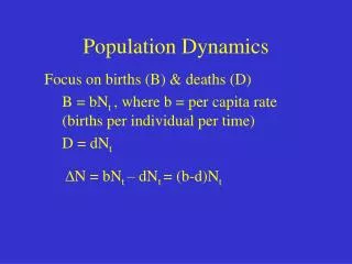
Population Attributes • Density – number of organisms per unit area or per unit volume • Affected by: • Natality – the reproductive output (birth rate) of a population • Mortality – the death rate of organisms in a population • Immigration – number of organisms moving into the area occupied by the population • Emigration – number of organisms moving out of the area occupied by the population
Population Density Four primary population parameters:
Unitary and Modular Organisms • Unitary organisms – individual units such as humans or mice • Modular organisms – organisms that do not come in simple units of individuals • Several grasses that are attached by runners
Density Examples Two fundamental attributes that affect our choice of techniques for population estimation are the size and mobility of the organism with respect to humans.
Abundance and Animal Size Birds are less abundant than mammals of equivalent size.
Two Types of Density Estimates • Absolute Density – a known density such as #/m2 • Relative Density – we know when one area has more individuals than another
Measuring Absolute Density • Total Count – count the number of organisms living in an area • Human census, number of oak trees in a wooded lot, number of singing birds in an area • Total counts generally are not used very often • Sampling Methods – use a sample to estimate population size • Either use the quadrat or capture-recapture method
Quadrat Method • A Quadrat is a sampling area of any shape randomly deployed. Each individual within the quadrat is counted and those numbers are used to extrapolate population size. • Example: a 100 square centimeter metal rectangle is randomly thrown four times and all of the beetles of a particular species within the square are counted each time: 19, 21, 17, and 19. This translates to 19 beetles per 100 cm2 or 1900 per m2.
Transects as Quadrats • Each transect was 110 meters long and 2m wide (220 m2 or 0.022/ha). All trees taller than 25 cm counted.
Capture-recapture Method • Important tool for estimating density, birth rate, and death rate for mobile animals. • Method: • Collect a sample of individuals, mark them, and then release them • After a period, collect more individuals from the wild and count the number that have marks • We assume that a sample, if random, will contain the same proportion of marked individuals as the population does • Estimate population density
Marked animals in second sample Marked animals in first sample Total caught in second sample Total population size 5 16 20 N Peterson Method = = N = 64
Assumptions For All Capture-Recapture Studies • Marked and unmarked animals are captured randomly. • Marked animals are subject to the same mortality rates as unmarked animals. The Peterson method assumes no mortality during the sampling period. • Marked animals are neither lost or overlooked.
Indices of Relative Density • Assume that samples represent some relatively constant but unknown relationship to total population size. • # cars in the Piggly Wiggly parking lot • Provides an index of abundance • Is population increasing, decreasing, or staying the same • Are there more animals in one location than another? • Can not quantify differences between sites • Twice the number of tracks does not = twice as many animals
Traps Number of Fecal Pellets Vocalization Frequency Pelt Records Catch per Unit Fishing Effort Number of Artifacts Questionnaires Cover Feeding Capacity Roadside Counts Some Indices Used
Natality • Fecundity – physiological notion that refers to an organism’s potential reproductive potential • Usually inversely proportional to the amount of parental care given to young • Fertility – Ecological concept that is based on the number of viable offspring produced during a specific period • Realized fertility – actual fertility rate • One birth per 15 years per human female in the child-bearing ages • Potential fertility – potential fertility rate • One birth per 10 to 11 months per human female in the child-bearing ages
Mortality • Opposite of mortality is survival • Longevity focuses on the age of death of individuals in a population • Potential longevity – maximum lifespan by an individual of a particular species • Set by the organisms physiology (dies of old age) • Sometimes described as the average longevity of individuals living in optimal conditions • Realized longevity – actual life span of an organism • Measured as an average for all animals living under real environmental conditions
Determining Mortality • Mark several individuals and measure how many survive from time t to t+1. • If abundance of successive age groups is known, then you can estimate mortality between successive age groups. • Can use catch curves for fish: Or develop regression equation 292 Survival between age 2 and 3= 147/292=0.50 147
Immigration and Emigration • Seldom measured • Assumed to be equal or insignificant (island pop’s) • However, dispersal may be a critical parameter in population changes
Limitations of the Population Approach • How to determine what exactly is a population • How clear are the boundaries? • Population does not exist as an isolate • Individuals interact with other members of the community
Life Tables - Mortality • Mortality is one of the four key parameters that drive population changes. • We can use a life table to answer particular questions about population mortality rates. • What life stage has the highest mortality? • Do older organisms die more frequently than young organisms • A cohortlife table is an age-specific summary of the mortality rates operating on a cohort of individuals. • Cohort – a collective group of individuals • Fish year class, all mice born in March, tadpoles from a single frog, freshman year class
X = age nx = number alive at time t lx = proportion of organisms surviving from the start of the lifetable to age x (ex: l1 = n1/n0, 0.217 =25/115; l2=n2/n0, 0.165=19/115) dx = number dying during the age interval x to x + 1 (ex:d0=n0-n1, 90 = 115-25; d1=n1-n2, 6=25-19) qx = per capita rate of mortality during the age interval x to x + 1 (ex: q0=d0/n0, 0.78 =90/115; q1=d1/n1) Cohort Life Table:
Formula’s For Cohort Life Table • X = age group we decide on • nx = observed • lx = lx+1 = nx+1/nx (overall survival) • dx = nx - nx+1 (age specific number dying) • qx = dx / nx (age specific mortality rate)
Per Capita Rates • Per capita is a presentation of data as a proportion of the population. • Suppose a disease kills 400 ducks: • If total duck population = 250,000 then the per capita mortality = 400/250,000 = 0.16%. • If total duck population = 2,500 then the per capita mortality = 400/2,500 = 16%. • Per capita gives us an idea of how the entire population is affected.
Survivorship Curve A plot of nx on a Log scale from a starting cohort of 1,000 individuals.
Three Types of General Curves Survival curve • Examples of Each Type: • Type 1 – Humans • Type 2 – Birds • Type 3 - Fish These curves are models. Most real curves are intermediate. Mortality curve
Static Life Table Calculated by taking a cross section of a population at a specific time: Per Capita
Cohort Versus Static Life Tables • Cohort follows an individual cohort through time and static looks at all of the individuals currently present. • The two are equal if and only if the environment does not change from year to year and the population is at equilibrium. • The human cohort life table for 1900 does little good for predicting life expectancy for today.
How to Collect Life Table Data • Survivorship directly observed. • Follow an individual cohort through time at close intervals. • Best to have since it generates a cohort life table directly and does not assume that the population is stable over time. Balanus can affect the survival of Chthamalus as determined by survivorship curve
How to Collect Life Table Data • Age at Death Observed. • By determining how old individuals were when they died, we can create a life table. Based on 584 individuals plus observed estimated mortality for age 1 and 2 individuals
How to Collect Life Table Data • Age Structure Directly Observed. • We can construct a life table based on the age structure of a population • Counting rings on a tree or a fish otolith. • Assume a constant age structure, which is hardly the case.
Mortality Rate (qx) Aging • Does mortality increase with age (senescence)? • Not for some Mediterranean fruit flies: This data proves our simple theory of senescence is not correct
Intrinsic Capacity For Increase In Numbers • By combining reproduction and mortality estimates, we can determine net population change (intrinsic capacity for increase). • The environment can influence population mean longevity or survival rate, natality rate, and growth rate. • Can be summed with natality and death rate
Fertility Schedule Population net reproductive rate 0.6% increase each generation bx = natality (lx)(bx) = reproductive output for that age class R0 < 1 population is declining, R0 = 1 population is stable, R0 > population is increasing.
Population Increase • If survival and fertility rates do not change, and no limit is placed on population growth – at what rate will a population increase? • It seems we need to know age-specific survival rates, age-specific fertility rates, and age structure • If all females in U.S. were >50 years old, no new young would be produced. • However, the age structure does not need to be known!
Stable Age Distribution • Given constant schedule of natality and mortality rates, a population will eventually reach a stable age distribution, and will remain at this age distribution indefinitely. • Stable age distribution: • 60% age 0 • 25% age 1 • 10% age 2 • 4% age 3 • Although the absolute number will change, the proportion of each age class remains constant!
For Example This animal lives three years, produces two young at exactly one year, and one young at exactly year two, and no young year three, then dies at end of year 3. If a population starts with one individual at age 0, the age distribution quickly becomes stable: 60% age 0, 25% age 1, 10% age 2, and 4% age 3.
dN Written in integral form Nt = N0ert rN = dt Stable Age Distribution When a population has reached the stable age distribution, it will increase in numbers according to: Nt = number of individuals at time t N0 = number of individuals at time 0 e = 2.71828 (a constant) r = intrinsic capacity for increase for the particular environmental conditions t = time This equation describes the curve of geometric increase in an expanding population (or geometric decrease to zero if r is negative).
For Example: N0ert =Nt Any population on a fixed age schedule of natality and mortality will change geometrically. This geometric change will dictate a fixed and unchanging age distribution – the stable age distribution.
lxbxx Gc = Ro Generation Time • Generation time – mean period elapsing between the production or ‘birth’ of parents and the production or ‘birth’ of offspring. • We can calculate generation time from a life table:
loge(3.0) loge(R0) r = = = 0.824 per individual per year G 1.33 Calculating r from a life table: Gc = 4.0/3.0 = 1.33 years lxbxx = 4.0 r > 0 population increasing, r = 0 population stable, r < 0 population decreasing
lx = proportion of original individuals surviving to each age class. bx = number of offspring produced per individual for the given age class (often refers to females only) R0 = net reproductive output (lxbx) > 1 pop increasing, = 1 pop stable, < 1 pop decreasing Gives us a multiplier to see how much the population increases each generation Gc= generation time this is an approximation because not all births occur at once. r = the populations intrinsic capacity for increase each r is for a specific set of environmental conditions environmental conditions may affect survival/reproduction > 0 pop increasing, = 0 pop stable, < 0 pop decreasing
Temperature and moisture effects on r value for a wheat beetle (Store wheat in cool dry place). Comparison of r value’s for two species of wheat beetle.
Species With a High r • Are not necessarily more common • However, these species can recover more quickly from disturbances
Increasing r: r = R0/G • Reduction in age at first reproduction • Basically reduce generation time • Increase the number of progeny in each reproductive event • Increases R0 • Increase the number of reproductive events • Increase in longevity essentially increases R0
About r • r is an oversimplification of nature • We do not find populations with a stable age distribution or with constant age-specific mortality and fertility rates • Actual population increases we observed varies in more complex ways than the theoretical r • However, the importance of r lies mostly in its use as a model for comparison with the actual rates of increase we see in nature • Can be used to assess environmental quality
ltbt ltbt w w Vx = Vx = bx + t=x lx lx t=x+1 Reproductive Value • Reproductive value – the contribution to the future population that an individual will make • In a stable population reproductive value at age x = or t and x are age and w is age of last reproduction
Females begin breeding Males protect harems