Recap from Friday
Recap from a CS195g Computational Photography lecture discussing Fourier Transform in image processing, filtering techniques, convolution, and boundary conditions. Learn about frequency domain, Fourier series, filtering types, Laplacian Pyramid, image gradient, and DCT in JPEG compression.


Recap from Friday
E N D
Presentation Transcript
Recap from Friday linear Filtering convolution differential filters filter types boundary conditions.
The Frequency Domain Somewhere in Cinque Terre, May 2005 CS195g: Computational Photography James Hays, Brown, Spring 2010 Slides from Steve Seitzand Alexei Efros
Salvador Dali “Gala Contemplating the Mediterranean Sea, which at 30 meters becomes the portrait of Abraham Lincoln”, 1976 Salvador Dali, “Gala Contemplating the Mediterranean Sea, which at 30 meters becomes the portrait of Abraham Lincoln”, 1976 Salvador Dali, “Gala Contemplating the Mediterranean Sea, which at 30 meters becomes the portrait of Abraham Lincoln”, 1976
A nice set of basis Teases away fast vs. slow changes in the image. This change of basis has a special name…
Jean Baptiste Joseph Fourier (1768-1830) • had crazy idea (1807): • Any periodic function can be rewritten as a weighted sum of sines and cosines of different frequencies. • Don’t believe it? • Neither did Lagrange, Laplace, Poisson and other big wigs • Not translated into English until 1878! • But it’s true! • called Fourier Series
A sum of sines • Our building block: • Add enough of them to get any signal f(x) you want! • How many degrees of freedom? • What does each control? • Which one encodes the coarse vs. fine structure of the signal?
Inverse Fourier Transform Fourier Transform F(w) f(x) F(w) f(x) Fourier Transform • We want to understand the frequency w of our signal. So, let’s reparametrize the signal by w instead of x: • For every w from 0 to inf, F(w) holds the amplitude A and phase f of the corresponding sine • How can F hold both? Complex number trick! We can always go back:
Time and Frequency • example : g(t) = sin(2pf t) + (1/3)sin(2p(3f) t)
Time and Frequency • example : g(t) = sin(2pf t) + (1/3)sin(2p(3f) t) = +
Frequency Spectra • example : g(t) = sin(2pf t) + (1/3)sin(2p(3f) t) = +
Frequency Spectra • Usually, frequency is more interesting than the phase
Frequency Spectra = + =
Frequency Spectra = + =
Frequency Spectra = + =
Frequency Spectra = + =
Frequency Spectra = + =
Extension to 2D in Matlab, check out: imagesc(log(abs(fftshift(fft2(im)))));
The greatest thing since sliced (banana) bread! The Fourier transform of the convolution of two functions is the product of their Fourier transforms The inverse Fourier transform of the product of two Fourier transforms is the convolution of the two inverse Fourier transforms Convolution in spatial domain is equivalent to multiplication in frequency domain! The Convolution Theorem
2D convolution theorem example |F(sx,sy)| f(x,y) * h(x,y) |H(sx,sy)| g(x,y) |G(sx,sy)|
Low-pass, Band-pass, High-pass filters low-pass: High-pass / band-pass:
What does blurring take away? original
What does blurring take away? smoothed (5x5 Gaussian)
High-Pass filter smoothed – original
Band-pass filtering • Laplacian Pyramid (subband images) • Created from Gaussian pyramid by subtraction Gaussian Pyramid (low-pass images)
Laplacian Pyramid • How can we reconstruct (collapse) this pyramid into the original image? Need this! Original image
Why Laplacian? Gaussian Laplacian of Gaussian delta function
- = + a = Unsharp Masking
The gradient direction is given by: • how does this relate to the direction of the edge? • The edge strength is given by the gradient magnitude Image gradient • The gradient of an image: • The gradient points in the direction of most rapid change in intensity
Effects of noise • Consider a single row or column of the image • Plotting intensity as a function of position gives a signal How to compute a derivative? Where is the edge?
Look for peaks in Solution: smooth first Where is the edge?
Derivative theorem of convolution • This saves us one operation:
Laplacian of Gaussian • Consider Laplacian of Gaussian operator Where is the edge? Zero-crossings of bottom graph
Laplacian of Gaussian is the Laplacian operator: 2D edge detection filters Gaussian derivative of Gaussian
Try this in MATLAB • g = fspecial('gaussian',15,2); • imagesc(g); colormap(gray); • surfl(g) • gclown = conv2(clown,g,'same'); • imagesc(conv2(clown,[-1 1],'same')); • imagesc(conv2(gclown,[-1 1],'same')); • dx = conv2(g,[-1 1],'same'); • imagesc(conv2(clown,dx,'same')); • lg = fspecial('log',15,2); • lclown = conv2(clown,lg,'same'); • imagesc(lclown) • imagesc(clown + .2*lclown)
Depends on Color R G B
Lossy Image Compression (JPEG) Block-based Discrete Cosine Transform (DCT)
Using DCT in JPEG • The first coefficient B(0,0) is the DC component, the average intensity • The top-left coeffs represent low frequencies, the bottom right – high frequencies
Image compression using DCT • DCT enables image compression by concentrating most image information in the low frequencies • Lose unimportant image info (high frequencies) by cutting B(u,v) at bottom right • The decoder computes the inverse DCT – IDCT • Quantization Table • 3 5 7 9 11 13 15 17 • 5 7 9 11 13 15 17 19 • 7 9 11 13 15 17 19 21 • 9 11 13 15 17 19 21 23 • 11 13 15 17 19 21 23 25 • 13 15 17 19 21 23 25 27 • 15 17 19 21 23 25 27 29 • 17 19 21 23 25 27 29 31
Block size in JPEG • Block size • small block • faster • correlation exists between neighboring pixels • large block • better compression in smooth regions • It’s 8x8 in standard JPEG
JPEG compression comparison 89k 12k