Download
1 / 20
200 likes | 410 Vues
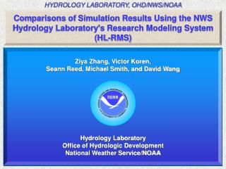
Overview of NWS Distributed Model (HL-RDHM). Mike Smith Victor Koren, Seann Reed, Zhengtao Cui, Ziya Zhang, Fekadu Moreda, Yu Zhang. Model Structure. Operational Version. HL-RDHM. P& ET. P, T & ET. Auto Calibration. SNOW -17. rain. rain + melt. SAC-SMA. SAC-SMA, SAC-HT.

E N D
Overview of NWS Distributed Model (HL-RDHM) Mike Smith Victor Koren, Seann Reed, Zhengtao Cui, Ziya Zhang, Fekadu Moreda, Yu Zhang
Model Structure Operational Version HL-RDHM P& ET P, T & ET Auto Calibration SNOW -17 rain rain + melt SAC-SMA SAC-SMA, SAC-HT surface runoff surface runoff base flow base flow Hillslope routing Hillslope routing Channel routing Channel routing Mods Flows and state variables Flows and state variables Calibration Forecasting
Sacramento Soil Moisture Accounting Model Courtesy of U. Arizona
UZFWC UZFWC UZTWC UZTWC LZFPC LZFPC LZFSC LZFSC LZTWC LZTWC 1. Modified Sacramento Soil Moisture Accounting Model In each grid and in each time step, transform conceptual soil water content to physically-based water content SAC-HT Physically-based Soil Layers and Soil Moisture Sacramento Model Storages Sacramento Model Storages SMC1 SMC2 SMC3 SMC4 SMC5 Soil moisture Soil temperature
Observed (white) and simulated (red) soil temperature and moisture at 20cm, 40cm, and 80cm depths. Valdai, Russia, 1971-1978 Soil Moisture Soil Temperature
2. Soils Data for SAC Parameters Demonstration of scale difference between polygons in STATSGO and SSURGO SSURGO STATSGO
2. SAC-SMA Parameters Objective estimation procedure:produce spatially consistent and physically realistic parameter values 1. Based on STATSGO; CN = f (hydro soil group only) • Assumed “pasture or range land use” under “fair” hydrologic conditions • National coverage • Available now via CAP 2. Based on STATSGO; CN = f(hydro soil group, landuse) • Global Land Cover Characterization (GLCC, 1 km) • National coverage • Being evaluated • Based on SSURGO; CN = f(hydro soil group, landuse) • National Land Cover Database (NLCD, 30 m) • Parameters for 25 states so far • Being evaluated
3. Routing Model Real HRAP Cell Hillslope model Cell-to-cell channel routing
3. Channel Routing Model • Uses implicit finite difference solution technique • Solution requires a unique, single-valued relationship between cross-sectional area (A) and flow (Q) in each grid cell (Q=q0Aqm) • Distributed values for the parameters q0 and qm in this relationship are derived by using • USGS flow measurement data at selected points • Connectivity/slope data • Geomorphologic relationships
4. Manual and Auto Calibration • Start with lumped calibration • Adjustment of parameter scalar multipliers • Use manual and auto adjustment as a strategy • Parameters optimized: • SAC-SMA • Hillslope and channel routing • Search algorithms • Simple local search: Kuzmin, Seo, and Koren, 2007. “Fast and Efficient Optimization of Hydrologic Model Parameters Using a Priori Estimates and Stepwise Line Search” Journal of Hydrology, in review • Objective function: Multi-scale
42 21 36 48 18 24 32 62 56 32 16 31 28 16 42 30 44 40 21 15 22 20 42 21 44 22 40 20 Calibration Approach Multiply each grid value by the same scalar factor. x 2 = Preserve Spatial Pattern of Parameters Example: I parameter out of N total model parameters th Calibrate distributed model by uniformly adjusting all grid values of each model parameter (i.e., multiply each parameter grid value by the same factor) 1. Manual: manually adjust the scalar factors to get desired hydrograph fit. 2. Auto: use auto - optimization techniques to adjust scalar factors .
HL-RDHM P, T & ET SNOW -17 rain + melt Auto Calibration SAC-SMA, SAC-HT surface runoff Execute these components in a loop to find the set of scalar multipliers that minimize the objective function base flow Hillslope routing Channel routing Flows and state variables
Multi-Scale Objective Function (MSOF) Emulates multi-scale nature of manual calibration • Minimize errors over hourly, daily, weekly, monthly intervals (k=1,2,3,4…n…userdefined) • q = flow averaged over time interval k • n = number of flow intervals for averaging • mk = number of ordinates for each interval • X = parameter set Weight: -Assumes uncertainty in simulated streamflow is proportional to the variability of the observed flow -Inversely proportional to the errors at the respective scales. Assume errors approximated by std. =
Calibration: MSOF Time Scales Average monthly flow Average weekly flow Average daily flow Multi-scale objective functionrepresents different frequencies of streamflow and its use partially imitates manual calibration strategy Hourly flow
Auto Calibration: Case 1 Example of HL-RDHM Auto Calibration: ELDO2 for DMIP 2 Arithmetic Scale After auto calibration Before Auto calibration of a priori parameters Observed
Auto Calibration: Case 1 Example of HL-RDHM Auto Calibration: ELDO2 for DMIP 2 Semi-Log Scale Observed After auto calibration Before Auto calibration of a priori parameters
Auto Calibration: Case 2 Example of HL-RDHM Auto Calibration: ELDO2 for DMIP 2 Arithmetic Scale After autocalibration Before Auto calibration of a priori parameters Observed
How much do the parameters change? Example for SLOA4
OHD Spatial and Temporal Scales for DMIP2 • “OHD” simulations • HRAP (~ 4 km) pixels for water balance calculations • Pixel main channels subdivided for accurate routing (usually 4 subreaches) • Basic time step: hourly (SAC percolation, hillslope routing, and channel routing functions may automatically shorten the time step under certain conditions) • Climatological PE and PE adjustments used (PE mid-month data interpolated to generate smoothly varying daily inputs) • “OH2” simulations • ½ HRAP pixel simulations for TALO2 and interior points only
References • Koren et al., 2004. “Hydrology Laboratory Research Modeling System (HL-RMS) of the US National Weather Service” Journal of Hydrology, 291, 297-318 • Koren, 2005. “Physically-Based Parameterization of Frozen Ground Effects: Sensitivity to Soil Properties” VIIth IAHS Scientific Assembly, Session 7.2, Brazil, April. • Koren, 2003. Parameterization of Soil Moisture-Heat Transfer Processes for Conceptual Hydrological Models”, paper EAE03-A-06486 HS18-1TU1P-0390, AGU-EGU, Nice, France, April. • Mitchell, K., Koren, others, 2002. “Reducing near-surface cool/moist biases over snowpack and early spring wet soils in NCEP ETA model forecasts via land surface model upgrades”, Paper J1.1, 16th AMS Hydrology Conference, Orlando, Florida, January • Koren et al., 1999. “A parameterization of snowpack and frozen ground intended for NCEP weather and climate models”, J. Geophysical Research, 104, D16, 19,569-19,585. • Koren, et al., 1999. “Validation of a snow-frozen ground parameterization of the ETA model”, 14th Conference on Hydrology, 10-15 January 1999, Dallas, TX, by the AMS, Boston MA, pp. 410-413. • http://www.nws.noaa.gov/oh/hrl/frzgrd/index.html