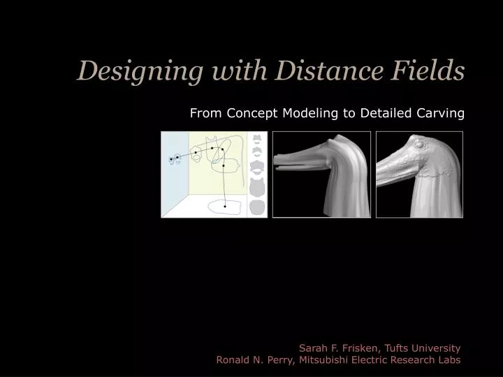

Designing with Distance Fields
E N D
Presentation Transcript
Designing with Distance Fields From Concept Modeling to Detailed Carving Sarah F. Frisken, Tufts University Ronald N. Perry, Mitsubishi Electric Research Labs
Distance Fields • An object’s distance field represents, for any point in space, the distance from that point to the object • The distance can be signed to distinguish between the inside and outside of the object Outside Boundary of shape Inside 2D Shape Shape’s distance field
Distance Fields • Distance fields are implicit representations of shape … • See Introduction to Implicit Surfaces (J. Bloomenthal, ed.), 1997 • The surface of the shape is an implicit surface • An implicit surface is an iso-contour of an implicitly defined scalar function
Distance Fields • An example of an implicit representation, F(x), where x 3 A 2D cross section of F(x) An iso-contour of F(x) where F(x) = 0.28
Distance Fields • Typically, for a shape represented by a distance field, the shape’s boundary, W, is the zero-valued iso-surface of the distance function • i.e., for an implicitly defined distance function, dist(x),W is the set of all points where dist(x) = 0
Distance Fields • General distance function dist(x) = Norm(x - S(x)), where Norm(u) is a metric that decreases monotonically with ||u||, and S(x) is a point on the boundary W • Minimum distance S(x) = s*,wheres* is on W and |Norm(x-s*)| |Norm(x - S)|,SW • Euclidean norm • Minimum Euclidean distance dist(x) = √(x – s*) (x– s*) T) = √(x – sx*)2 + (y – sy*) 2 + (z – sz*) 2, for x = (x, y, z) = the signed magnitude of the vector from x to s*
General Properties • Distance fields are defined every where in space • Not just on the surface like boundary representations • It is trivial to determine whether a point is inside, outside or on the boundary of a shape • Evaluate F(x) and compare it to the value of the iso-surface • Gradients of the distance field provide geometric information • On the surface • The gradient is normal to the surface • Off the surface • The gradient points in the direction of the closest surface point
Continuity Properties • Distance fields are C0 continuous everywhere • Euclidean distance fields are C1 continuous except at boundaries of Voronoi Regions • C1 near smooth sections of the boundary • Distance field is linear near linear sections of the boundary • Not C1 near corners or the medial axis Distance field is C0 continuous C1 continuous except at Voronoi boundaries
Operations on Distance Fields • Constructive Solid Geometry or CSG is the result of a Boolean operations applied to primitive, aggregate, or CSG objects • Boolean operations on distance fields are fast and simple A B A B A B Union: A B Intersection: A B Difference: A – B
Operations on Distance Fields • Boolean operations are fast and simple Intersection: dist(A B) = min (dist(A), dist(B)) Union: dist(A B) = max (dist(A), dist(B)) Difference: dist(A - B) = min (dist(A), –dist(B))
Operations on Distance Fields • Boolean operations are fast and simple Union of two shapes Union of two distance fields
Advantages • Conceptual advantages over outlines • Distance fields represent more than just the object outline • Represent the object interior, exterior, and its boundary (useful for CSG operations and physical simulation) Exterior Boundary of shape Interior Shape’s distance field
Advantages • Conceptual advantages over outlines • Distance fields represent more than just the object outline • Represents an infinite number of offset surfaces Boundary offsets
A B A’ B’ A B A’ B’ Advantages • Conceptual advantages over outlines • Gains in efficiency and quality because distance fields vary smoothly (C0 continuous) and throughout space Intensity profile of the distance field is C0 continuous throughout space Intensity profile of the standard representation is discontinuous at boundaries
Advantages • Conceptual advantages over outlines • Gradient of the distance field yields • Surface normal for points on the edge • Direction to the closest edge point for points off the edge Point off the edge Point on the edge
History – Rendering and Processing • Distance fields are a specific example of implicit functions (see “Introduction to Implicit Surfaces”, ed. Bloomenthal, 1997) • Rendering and processing • Tessellation • Bloomenthal, “Polygonization of Implicit Surfaces”, Computer Aided Geometric Design, 1988 • Szeliski and Tonnesen, “Surface modeling with oriented particle systems”, SIGGRAPH, 1992 • Heckbert and Witkin, “Using particles to sample and control implicit surfaces”, SIGGRAPH, 1994 • Ray tracing • Zuiderveld et al., “Acceleration of Ray-Casting using 3D Distance Transforms”, Vis. In Biomedical Computing, 1992 • Yagel and Shi, “Accelerating Volume Animation by Space-Leaping”, IEEE Vis. 1993
History – Applications • CAD • Offsetting • Ricci, “A Constructive Geometry for Computer Graphics”, Computer, 1973 (CSG of implicit representations of solids • Breen, “Constructive Cubes: CSG Evaluation for Display Using Discrete 3D Scalar Data Sets”, Eurographics, 1991 • Tolerancing • Requicha, “Towards a Theory of Geometric Tolerancing”, J. Robotics Research, 1983 • Rounds and filets • Rockwood, “The Displacement Method for Implicit Blending in Solid Models”, Transactions on Graphics, 1989 • Swept surfaces and volumes • Schroeder, Lorensen, and Linthicum, “Implicit Modeling of Swept Surfaces and Volumes”, IEEE Vis. 1994 • Simulation • Biswas and Shapiro, “Approximate distance fields with non-vanishing gradients”, Graphical Models, 2004
History – Applications • Image processing • Image segmentation • Yang , Staib, and Duncan, " Neighbor-Constrained Segmentation with Level Set Based 3D Deformable Models,“ IEEE Trans Med Imaging, 2004 • e.g., watershed segmentation • Shape matching • Lavalle and Szeliski, “Recovering the Position and Orientation of Free Form Objects from Image Contours Using 3D Distance Maps”, IEEE PAMI, 1995 Original image, watershed segmentation, and segmented cells: from www.cellprofiler.org
History – Applications • Medical • 3D surface reconstruction from cross sections • Raya and Udupa, “Shape-based Interpolation of Multi-dimensional Objects”, IEEE Trans. Med. Imaging, 1990 • Navigation during virtual surgery • Hong, et. al, “Virtual Voyage: Interactive Navigation in the Human Colon”, SIGGRAPH 1997 • Medial axis representation for animation of the Virtual Human • Gagvani and Silver, Animating volumetric models, Graphical Models, 2001 Animating the Virtual Human: from Gagvani and Silver, 2001
History – Applications • Robotics • Path planning • Lengyel et al., “Real-time Robot Motion Planning Using Rasterizing Computer Graphics Hardware”, SIGGRAPH 1990 • Collision detection • Fisher and Lin, “Deformed Distance Fields for Simulation of Non-Penetrating Flexible Bodies”, Eurographics Wkshop on Comp Anim and Modeling, 2001 • Haptics • Gibson et al, “Simulating Arthroscopic Knee Surgery using Volumetric Object Representations, Real-time Volume Rendering, and Haptic Feedback", CVRMed, 1997
History – Applications • Simulation • Modeling continually varying heterogeneous materials • Biswas, Shapiro, and Tsukanov. Heterogeneous Material Modeling with Distance Fields. Technical Report, 2002-4. • Level sets • Osher and Sethian, “Fronts Propagating with Curvature-Dependent Speed, Algorithms Based on Hamilton-Jacobian Formulation”, J. Computational Physics, 1988 Fedkiw, Stam, and Jensen Neuyen, Fedkiw, and Jensen Enright, Marschner, and Fedkiw
History – Applications • Reconstructing 3D models from range data • Unorganized points, projected distances, 3D distance fields • Hoppe et al., “Surface Reconstruction from Unorganized Points”, SIGGRAPH, 1992 • Bajaj, Bernardini, and Xu, “Automatic Reconstruction of Surfaces and Scalar Fields from 3D Scans”, SIGGRAPH 1995 • Curlass and Levoy, “A volumetric Method for Building Complex Models from Range Images”, SIGGRAPH 1996 • Carr et al., “Reconstruction and Representation of 3D Objects with Radial Basis Functions”, SIGGRAPH 2001 • Hilton et al., “Reliable Surface Reconstruction from Multiple Range Images”, European Conf. on Computer Vision, 1996 • Wheeler et al., “Consensus Surfaces for Modeling 3D Objects from Multiple Range Images”, Int. Conf. on Computer Vision, 1998 • Whitaker, “A Level-set Approach to 3D Reconstruction from Range Data”, International J. Computer Vision, 1998 • Boissonnat and Cazals, “Smooth Surface Reconstruction via Natural Neighbor Interpolation of Distance Functions”, ACM Symposium on Computational Geometry, 2000 • Sagaawa, Nishino, and Ikeuchi, “Robust and Adaptive Integration of Multiple Range Images with Photometric Attributes”, 2001 • Frisken and Perry, “Efficient Estimation of 3D Euclidean Distance Fields from 2D Range Images", Symposium on Volume Visualization, 2002
History – Applications • Distance Fields for Design • Bloomenthal and Wyville, Interactive Techniques for Implicit Modeling”, Computer Graphics, 1990
History – Applications • Distance Fields for Design • Gaylean and Hughes, “Sculpting: an Interactive Volume Modeling Technique”, SIGGRAPH 1991
History – Applications • Distance Fields for Design • Avila and Sobierajski, “A Haptic Interaction Method for Volume Visualization, IEEE Visualization 1996
History – Applications • Distance Fields for Design • Wang and Kaufman, “Volume Sculpting”, Interactive 3D Graphics, 1995.
History – Applications • Distance Fields for Design • Baerentzen, “Octree-based Volume Sculpting, IEEE Symposium on Vol. Vis., 1998
History – Applications • Distance Fields for Design • Cani (Gascuel), “An Implicit Formulation for Precise Contact Modeling Between Flexible Solids”, SIGGRAPH 1993
History – Applications • Distance Fields for Design • Desbrun and Cani, “Active Implicit Surface for Animation”, Graphics Interface, 1998
History – Applications • Distance Fields for Design • Blanch, Ferley, Cani, Gascuel “Non-Realistic Haptic Feedback for Virtual Sculpture”, Rapport de recherche RR-5090, 2004
History – Applications • Distance Fields for Design • Perry, Frisken, “Kizamu: a system for sculpting digital characters”, SIGGRAPH 2001
History – Applications • Distance Fields for Design • Perry, Frisken, “Kizamu: a system for sculpting digital characters”, SIGGRAPH 2001
History – Applications • Distance Fields for Design • Museth et al. “Level Set Surface Editing Operators”, SIGGRAPH 2002
Representing Distance Fields • Implicit representation • e.g., sphere, dist(x,y,z) = R - √(x – cx*)2 + (y – cy*) 2 + (z – cz*) 2 • Distances are computed at query points as needed for rendering or processing • Complex models can be represented via CSG • Precise but slow for complex models S R
Representing Distance Fields • Sampled volumes • Distances are computed and stored in a regular 3D grid • Distances at non-grid locations are interpolated • Payne and Toga, “Distance Field Manipulation of Surface Models”, IEEE Computer Graphics and Applications, 1992 -30 -20 10 A 2D shape and three signed distance values A regularly sampling of the distance field A 2D image depicting the distance field
Representing Distance Fields • Sampled volumes • Smooth surfaces are well represented by a relatively small number of samples • Frisken (Gibson), “Using Distance Maps for Smooth Surface Representation in Sampled Volumes”, IEEE Symposium on Vol Vis, 1998 Radius = 30 voxels 100 x 100 x 100 Radius = 3 voxels 10 x 10 x 10 Radius = 2 voxels 10 x 10 x 10 Radius = 1.5 voxels 10 x 10 x 10
Representing Distance Fields • Sampled volumes • For detailed models, the distance field must be sampled at high enough rates to avoid aliasing during reconstruction and rendering • Regularly sampled volumes have • Slow processing times • Large memory requirements • Limited resolution
Representing Distance Fields • Addressing memory requirements and processing speed • Speed up distance computation using approximating distance transforms • Jones and Satherley “Voxelisation: Modeling for Volume Graphics”, in Vision, Modeling, and Visualization, 2000 3 2 2 3 4 4 2 1 1 2 2 3 1 0 0 1 1 2 2 1 0 0 0 1 3 2 1 0 0 1 4 3 2 1 1 2 Binary 2D shape Chessboard distance
Representing Distance Fields • Addressing memory requirements and processing speed • Speed up distance computation using hardware • Hoff et al, “Fast Computation of Generalized Voronoi Diagrams Using Graphics Hardware”, SIGGRAPH 1997 • E.g., points 2D distance field of a point A 3D cone with its apex at the point has z-coordinates that correspond to the point’s distance field
Representing Distance Fields • Addressing memory requirements and processing speed • Speed up distance computation using hardware • Hoff et al, “Fast Computation of Generalized Voronoi Diagrams Using Graphics Hardware”, SIGGRAPH 1997 • e.g., lines 2D distance field of a line A 3D folded plate with its apex along the line has z-coordinates that correspond to the line’s distance field
Representing Distance Fields • Addressing memory requirements and processing speed • Fast distance computation using hardware • Hoff et al, “Fast Computation of Generalized Voronoi Diagrams Using Graphics Hardware”, SIGGRAPH 1997 Hardware-generated Voronoi diagram of a chevron shape Projected 3D geometry used to approximate the 2D distance field of the chevron
Representing Distance Fields • Addressing memory requirements and processing speed • Fast distance computation using hardware • Hoff et al, “Fast Computation of Generalized Voronoi Diagrams Using Graphics Hardware”, SIGGRAPH 1997 Using hardware generated distance fields t0 control particle dynamics
Representing Distance Fields • Addressing memory requirements and processing speed • Reducing the number of distance samples • Distance shells (compute accurate distances in a narrow region near the boundary) • Jones, “The Production of Volume Data from Triangular Meshes Using Voxelisation”, Computer Graphics Forum,1996 • Sramek and Kaufman, “Alias-free voxelization of geometric objects”, IEEE Trans on Vis and Computer Graphics, 1999 • Level sets for propagating accurate distances throughout the volume • Kimmel and Sethian, “Fast Marching Methods for Computing Distance Maps and Shortest Paths”, Tech report, U.C. Berkeley, 1996 • Breen, Mauch, and Whitaker, “3D Scan Conversion of CSG Models into Distance Volumes”, IEEE Symposium on Vol Vis, 1998
Representing Distance Fields • Addressing memory requirements and processing speed • Reducing the number of distance samples • Boundary-limited Octrees • Jones and Satherly, “Shape Representation using Space Filled Sub-Voxel Distance Fields”, IEEE International Conf. on Shape Modeling and Apps, 2001 • Strain, “Fast Tree-based Redistancing for Level Set Computations”, J. Computational Physics, 1999 • ADFs • Frisken, Perry, Rockwood, Jones, “Adaptively Sampled Distance Fields: a General Representation of Shape for Computer Graphics”, SIGGRAPH 2000 Boundary-limited quadtree
Representing Distance Fields • Addressing memory requirements and processing speed • Reducing the number of distance samples • Boundary-limited octrees and quadtrees • Jones and Satherly, “Shape Representation using Space Filled Sub-Voxel Distance Fields”, IEEE International Conf. on Shape Modeling and Apps, 2001 • Strain, “Fast Tree-based Redistancing for Level Set Computations”, J. Computational Physics, 1999 • ADFs • Frisken, Perry, Rockwood, Jones, “Adaptively Sampled Distance Fields: a General Representation of Shape for Computer Graphics”, SIGGRAPH 2000 Boundary-limited quadtree Detail-directed ADF
Adaptively Sampled Distance Fields • Detail-directed sampling of the distance field Sample at low rates where the distance field is smooth. Sample at higher rates only where necessary (e.g., near corners).
Adaptively Sampled Distance Fields • Detail-directed sampling of the distance field • High sampling rates only where needed • Fewer distance samples to compute • Less memory required • Faster to process • Spatial data structure • Fast localization for efficient processing • ADFs are defined very generally: they consist of • Adaptively sampled distance values ... • Organized in a spatial data structure ... • With a method for reconstructing the distance field from the sampled distance values
Various Instantiations of ADFs Example of a quadtree-based 2D ADF
Various Instantiations of ADFs Example of a wavelet-based 2D ADF
Various Instantiations of ADFs Example of a multi-resolution triangulation-based 2D ADF