Bayesian Reasoning
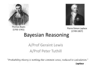
Bayesian Reasoning. A dapted from slides by Tim Finin. Thomas Bayes, 1701-1761. Today ’ s topics. Review probability theory Bayesian inference From the joint distribution Using independence/factoring From sources of evidence Bayesian Nets. Sources of Uncertainty.

Bayesian Reasoning
E N D
Presentation Transcript
BayesianReasoning Adapted from slides by Tim Finin Thomas Bayes, 1701-1761
Today’s topics • Review probability theory • Bayesian inference • From the joint distribution • Using independence/factoring • From sources of evidence • Bayesian Nets
Sources of Uncertainty • Uncertain inputs -- missing and/or noisy data • Uncertain knowledge • Multiple causes lead to multiple effects • Incomplete enumeration of conditions or effects • Incomplete knowledge of causality in the domain • Probabilistic/stochastic effects • Uncertain outputs • Abduction and induction are inherently uncertain • Default reasoning, even deductive, is uncertain • Incomplete deductive inference may be uncertain Probabilistic reasoning only gives probabilistic results (summarizes uncertainty from various sources)
Decision making with uncertainty Rationalbehavior: • For each possible action, identify the possible outcomes • Compute the probabilityof each outcome • Compute the utilityof each outcome • Compute the probability-weighted (expected) utilityover possible outcomes for each action • Select action with the highest expected utility (principle of Maximum Expected Utility)
Why probabilities anyway? Kolmogorov showed that three simple axioms lead to the rules of probability theory • All probabilities are between 0 and 1: 0 ≤ P(a) ≤ 1 • Valid propositions (tautologies) have probability 1, and unsatisfiable propositions have probability 0: P(true) = 1 ; P(false) = 0 • The probability of a disjunction is givenby: P(a b) = P(a) + P(b) – P(a b) a ab b
Random variables Domain Atomic event: complete specification of state Prior probability: degree of belief without any other evidence Joint probability: matrix of combined probabilities of a set of variables Alarm, Burglary, Earthquake Boolean (like these), discrete, continuous Alarm=TBurglary=TEarthquake=Falarm burglary ¬earthquake P(Burglary) = 0.1P(Alarm) = 0.1P(earthquake) = 0.000003 P(Alarm, Burglary) = Probability theory 101
Conditional probability: prob. of effect given causes Computing conditional probs: P(a | b) = P(a b) / P(b) P(b): normalizingconstant Product rule: P(a b) = P(a | b) * P(b) Marginalizing: P(B) = ΣaP(B, a) P(B) = ΣaP(B | a) P(a) (conditioning) P(burglary | alarm) = .47P(alarm | burglary) = .9 P(burglary | alarm) = P(burglary alarm) / P(alarm) = .09/.19 = .47 Probability theory 101 • P(burglary alarm) = P(burglary | alarm) * P(alarm) = .47 * .19 = .09 • P(alarm) = P(alarm burglary) + P(alarm ¬burglary) = .09+.1 = .19
Example: Inference from the joint P(burglary | alarm) = α P(burglary, alarm) = α [P(burglary, alarm, earthquake) + P(burglary, alarm, ¬earthquake) = α [ (.01, .01) + (.08, .09) ] = α [ (.09, .1) ] Since P(burglary | alarm) + P(¬burglary | alarm) = 1, α = 1/(.09+.1) = 5.26 (i.e., P(alarm) = 1/α = .19) P(burglary | alarm) = .09 * 5.26 = .474 P(¬burglary | alarm) = .1 * 5.26 = .526
Exercise:Inference from the joint • Queries: • What is the prior probability of smart? • What is the prior probability of study? • What is the conditional probability of prepared, given study and smart? P(prepared,smart,study)/P(smart,study) = 0.8 0.6 0.9
Independence • When sets of variables don’t affect each others’ probabilities, we call them independent, and can easily compute their joint and conditional probability: Independent(A, B) → P(AB) = P(A) * P(B), P(A | B) = P(A) • {moonPhase, lightLevel} might be independent of {burglary, alarm, earthquake} • Maybe not: crooks may be more likely to burglarize houses during a new moon (and hence little light) • But if we know the light level, the moon phase doesn’t affect whether we are burglarized • If burglarized, light level doesn’t affect if alarm goes off • Need a more complex notion of independence and methods for reasoning about the relationships
Exercise: Independence • Query: Is smart independent of study? • P(smart|study) == P(smart) • P(smart|study) = P(smart study)/P(study) • P(smart|study) = (.432 + .048)/(.432 + .048 + .084 + .036) = .48/.6 = 0.8 • P(smart) = .432 + .16 + .048 + .16 = 0.8 INDEPENDENT!
Conditional independence • Absolute independence: • A and B are independentif P(A B) = P(A) * P(B); equivalently, P(A) = P(A | B) and P(B) = P(B | A) • A and B are conditionally independentgiven C if • P(A B | C) = P(A | C) * P(B | C) • This lets us decompose the joint distribution: • P(A B C) = P(A | C) * P(B | C) * P(C) • Moon-Phase and Burglary are conditionally independent given Light-Level • Conditional independence is weaker than absolute independence, but still useful in decomposing the full joint probability distribution
Exercise: Conditional independence • Queries: • Is smart conditionally independent of prepared, given study? • P(smart prepared | study) == P(smart | study) * P(prepared | study) • P(smart prepared | study) = P(smart prepared study) / P(study) • = .432/ (.432 + .048 + .084 + .036) = .432/.6 = .72 • P(smart | study) * P(prepared | study) = .8 * .86 = .688 NOT!
Bayes’ rule • Derived from the product rule: • P(C | E) = P(E | C) * P(C) / P(E) • Often useful for diagnosis: • If E are (observed) effects and C are (hidden) causes, • We may have a model for how causes lead to effects (P(E | C)) • We may also have prior beliefs (based on experience) about the frequency of occurrence of effects (P(C)) • Which allows us to reason abductively from effects to causes (P(C | E))
Ex: meningitis and stiff neck • Meningitis (M) can cause a a stiff neck (S), though there are many other causes for S, too • We’d like to use S as a diagnostic symptom and estimate p(M|S) • Studies can easily estimate p(M), p(S) and p(S|M) p(S|M)=0.7, p(S)=0.01, p(M)=0.00002 • Applying Bayes’ Rule: p(M|S) = p(S|M) * p(M) / p(S) = 0.0014
Bayesian inference • In the setting of diagnostic/evidential reasoning • Know prior probability of hypothesis conditional probability • Want to compute the posterior probability • Bayes’s theorem (formula 1):
Simple Bayesian diagnostic reasoning • Also known as: Naive Bayes classifier • Knowledge base: • Evidence / manifestations: E1, … Em • Hypotheses / disorders: H1, … Hn Note: Ej and Hi are binary; hypotheses are mutually exclusive (non-overlapping) and exhaustive (cover all possible cases) • Conditional probabilities: P(Ej | Hi), i = 1, … n; j = 1, … m • Cases (evidence for a particular instance): E1, …, El • Goal: Find the hypothesis Hi with the highest posterior • Maxi P(Hi | E1, …, El)
Simple Bayesian diagnostic reasoning • Bayes’rule says that P(Hi | E1… Em) = P(E1…Em | Hi) P(Hi) / P(E1… Em) • Assume each evidence Ei is conditionally indepen-dent of the others, given a hypothesis Hi, then: P(E1…Em | Hi) = mj=1 P(Ej | Hi) • If we only care about relative probabilities for the Hi, then we have: P(Hi | E1…Em) = αP(Hi) mj=1 P(Ej | Hi)
Limitations • Cannot easily handle multi-fault situations, norcases where intermediate (hidden) causes exist: • Disease D causes syndrome S, which causes correlated manifestations M1 and M2 • Consider a composite hypothesis H1H2, where H1 and H2 are independent. What’s the relative posterior? P(H1 H2 | E1, …, El) = αP(E1, …, El | H1 H2) P(H1 H2) = αP(E1, …, El | H1 H2) P(H1) P(H2) = αlj=1 P(Ej | H1 H2)P(H1) P(H2) • How do we compute P(Ej | H1H2) ?
Limitations • Assume H1 and H2 are independent, given E1, …, El? • P(H1 H2 | E1, …, El) = P(H1 | E1, …, El) P(H2 | E1, …, El) • This is a very unreasonable assumption • Earthquake and Burglar are independent, but not given Alarm: • P(burglar | alarm, earthquake) << P(burglar | alarm) • Another limitation is that simple application of Bayes’s rule doesn’t allow us to handle causal chaining: • A: this year’s weather; B: cotton production; C: next year’s cotton price • A influences C indirectly: A→ B → C • P(C | B, A) = P(C | B) • Need a richer representation to model interacting hypotheses, conditional independence, and causal chaining • Next: conditional independence and Bayesian networks!
Summary • Probability is a rigorous formalism for uncertain knowledge • Joint probability distribution specifies probability of every atomic event • Can answer queries by summing over atomic events • But we must find a way to reduce the joint size for non-trivial domains • Bayes’ rule lets unknown probabilities be computed from known conditional probabilities, usually in the causal direction • Independenceand conditional independence provide the tools
Overview • Bayesian Belief Networks (BBNs) can reason with networks of propositions and associated probabilities • Useful for many AI problems • Diagnosis • Expert systems • Planning • Learning
BBN Definition • AKA Bayesian Network, Bayes Net • A graphical model (as a DAG) of probabilistic relationships among a set of random variables • Links represent direct influence of one variable on another source
Recall Bayes Rule Note the symmetry: we can compute the probability of a hypothesis given its evidence and vice versa.
P( S=no) 0.80 P( S=light) 0.15 P( S=heavy) 0.05 Smoking= no light heavy P( C=none) 0.96 0.88 0.60 P( C=benign) 0.03 0.08 0.25 P( C=malig) 0.01 0.04 0.15 Simple Bayesian Network Smoking Cancer
More Complex Bayesian Network Age Gender Exposure to Toxics Smoking Cancer Serum Calcium Lung Tumor
More Complex Bayesian Network Nodes represent variables Age Gender Exposure to Toxics Smoking Links represent “causal”relations Cancer • Does gender cause smoking? • Influence might be a more appropriate term Serum Calcium Lung Tumor
More Complex Bayesian Network predispositions Age Gender Exposure to Toxics Smoking Cancer Serum Calcium Lung Tumor
More Complex Bayesian Network Age Gender Exposure to Toxics Smoking condition Cancer Serum Calcium Lung Tumor
More Complex Bayesian Network Age Gender Exposure to Toxics Smoking Cancer observable symptoms Serum Calcium Lung Tumor
Independence Age and Gender are independent. Age Gender P(A,G) = P(G) P(A) P(A |G) = P(A) P(G |A) = P(G) P(A,G) = P(G|A) P(A) = P(G)P(A) P(A,G) = P(A|G) P(G) = P(A)P(G)
Conditional Independence Cancer is independent of Age and Gender given Smoking Age Gender Smoking P(C | A,G,S) = P(C|S) Cancer
Serum Calcium is independent of Lung Tumor, given Cancer P(L | SC,C) = P(L|C) P(SC | L,C) = P(SC|C) Conditional Independence: Naïve Bayes Serum Calcium and Lung Tumor are dependent Cancer Serum Calcium Lung Tumor Naïve Bayes assumption: evidence (e.g., symptoms) is indepen-dent given the disease. This makes it easy to combine evidence
Explaining Away Exposure to Toxics and Smoking are independent Exposure to Toxics Smoking Exposure to Toxics is dependent on Smoking, given Cancer Cancer P(E=heavy|C=malignant) > P(E=heavy|C=malignant, S=heavy) • Explaining away: reasoning pattern where confirmation of one cause of an event reduces need to invoke alternatives • Essence of Occam’s Razor
Conditional Independence A variable (node) is conditionally independent of its non-descendants given its parents Age Gender Non-Descendants Exposure to Toxics Smoking Parents Cancer is independent of Age and Gender given Exposure to Toxics and Smoking. Cancer Serum Calcium Lung Tumor Descendants
Another non-descendant A variable is conditionally independent of its non-descendants given its parents Age Gender Exposure to Toxics Smoking Diet Cancer Cancer is independent of Dietgiven Exposure toToxics and Smoking Serum Calcium Lung Tumor
BBN Construction The knowledge acquisition process for a BBN involves three steps • Choosing appropriate variables • Deciding on the network structure • Obtaining data for the conditional probability tables
KA1: Choosing variables Variables should be collectively exhaustive, mutually exclusive values Error Occurred No Error They should be values, not probabilities Risk of Smoking Smoking
Heuristic: Knowable in Principle Example of good variables • Weather {Sunny, Cloudy, Rain, Snow} • Gasoline: Cents per gallon • Temperature { 100F , < 100F} • User needs help on Excel Charting {Yes, No} • User’s personality {dominant, submissive}
Age Gender Exposure to Toxic Smoking Genetic Damage Cancer KA2: Structuring Network structure corresponding to “causality” is usually good. Initially this uses the designer’s knowledge but can be checked with data Lung Tumor
KA3: The numbers • Second decimal usually doesn’t matter • Relative probabilities are important • Zeros and ones are often enough • Order of magnitude is typical: 10-9 vs 10-6 • Sensitivity analysis can be used to decide accuracy needed
Three kinds of reasoning BBNs support three main kinds of reasoning: • Predicting conditions given predispositions • Diagnosing conditions given symptoms (and predisposing) • Explaining a condition in by one or more predispositions To which we can add a fourth: • Deciding on an action based on the probabilities of the conditions
Predictive Inference Age Gender How likely are elderly males to get malignant cancer? Exposure to Toxics Smoking P(C=malignant| Age>60, Gender=male) Cancer Serum Calcium Lung Tumor
Predictive and diagnostic combined Age Gender How likely is an elderly male patient with high Serum Calciumto have malignant cancer? Exposure to Toxics Smoking Cancer P(C=malignant| Age>60, Gender= male, Serum Calcium = high) Serum Calcium Lung Tumor
Smoking • If we then observe heavy smoking, the probability of exposure to toxics goes back down. Explaining away • If we see a lung tumor, the probability of heavysmoking and of exposureto toxics both go up. Age Gender Exposure to Toxics Smoking Cancer Serum Calcium Lung Tumor
Decision making • Decision - an irrevocable allocation of domain resources • Decision should be made so as to maximize expected utility. • View decision making in terms of • Beliefs/Uncertainties • Alternatives/Decisions • Objectives/Utilities
dry dry Regret in wet wet Relieved Perfect! out Disaster A Decision Problem Should I have my party inside or outside?
Value Function A numerical score over all possible states of the world allows BBN to be used to make decisions
Two software tools • Netica: Windows app for working with Bayes-ian belief networks and influence diagrams • A commercial product but free for small networks • Includes a graphical editor, compiler, inference engine, etc. • Samiam: Java system for modeling and reasoning with Bayesian networks • Includes a GUI and reasoning engine

