Probabilities: Key Concepts and Applications
Learn about discrete probability, sample space, events, probability distribution, basic properties, conditional probability, Bayes' theorem, independent events, and binomial trials with practical examples and quizzes.

Probabilities: Key Concepts and Applications
E N D
Presentation Transcript
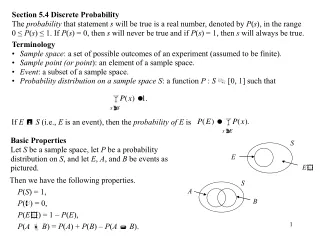
S E E S A B • Section 5.4 Discrete Probability • The probability that statement s will be true is a real number, denoted by P(s), in the range • 0 ≤ P(s) ≤ 1. If P(s) = 0, then s will never be true and if P(s) = 1, then s will always be true. • Terminology • Sample space: a set of possible outcomes of an experiment (assumed to be finite). • Sample point (or point): an element of a sample space. • Event: a subset of a sample space. • Probability distribution on a sample space S: a function P : S [0, 1] such that If ES (i.e., E is an event), then the probability of E is Basic Properties Let S be a sample space, let P be a probability distribution on S, and let E, A, and B be events as pictured. Then we have the following properties. P(S) = 1, P() = 0, P(E) = 1 – P(E), P(AB) = P(A) + P(B) – P(AB).
S A B Example. Two fair dice are tossed with sample space S = {(i, j) | i, j {1, 2, 3, 4, 5, 6}}. Since the dice are fair, P(i, j) = 1/36 for (i, j) S. Find the probability for each event. 1. The sum of dots is a prime number. 2. The sum of dots is not a prime number. 3. The sum of dots is greater than 4. Solution. Let E = {(1, 1), (1, 2), (2, 1), (1, 4), (4, 1), (1, 6), (6, 1), (2, 3), (3, 2), (2, 5), (5, 2), (3, 4), (4, 3), (5, 6), (6, 5)}. So | E | = 15. Therefore P(E) = 15(1/36) = 15/36. 2. Let E be the event of (1). Then P(E) = 1 – P(E) = 1 – 15/36 = 21/36. If E denotes the sum of dots greater than 4, then E = {(1, 1), (1, 2), (2, 1), (1, 3), (3, 1), (2, 2)}. So P(E) = 1 – P(E) = 1 – 6/36 = 30/36. Conditional Probability For events A and B where P(B) ≠ 0, the probability of A given B, written P(A | B), is: The idea for P(A | B) is to restrict the sample space to B as pictured. Note the following special cases: 1. If A B = , then P(A |B) = 0. 2. If B A, then P(A | B) = 1. 3. If A B, then P(A | B) = P(A)/P(B).
S B E1 E3 E2 Example. Toss two fair dice, as in the previous example. What is the probability that the top of the first die is 2 given that the sum of the two dice is 7? Solution. Let A be “the first die is 2” and let B be “the sum is 7”. Calculate P(A | B). A = {(2, 1), (2, 2), (2, 3), (2, 4), (2, 5), (2, 6)}, B = {(1, 6), (6, 1), (2, 5), (5, 2), (3, 4), (4, 3)}, Then A B = {(2, 5)}. So P(A | B) = P(A B)/P(B) = (1/36)/(6/36) = 1/6. Quiz. Toss two fair dice, as in the previous example. What is the probability that the top of the first die is less than 4 given that the sum of the two dice is less than 8? Answer. Let A be “the first die is less than 4” and let B be “the sum is less than 8”. Calculate P(A | B). B has 21 pairs, so P(B) = 21/36. A B contains those pairs in B that begin with 1, 2, or 3. So A B = {(1, 1), …, (1, 6), (2, 1), …, (2, 5), (3, 1), …, (3, 4)}, which has 15 pairs. So P(A B) = 15/36. Therefore P(A | B) = 15/21 = 5/7. Bayes’ Theorem Let S be partitioned by events E1, …, En, and let B be an event with P(B) ≠ 0 as pictured. The conditional probability P(Ei | B) can be thought of as the probability that B is caused byEi.
Example. Three chests C1, C2, and C3 each have 2 drawers. There is one coin in each drawer as follows: C1: gold and gold; C2: gold and silver; C3: silver and silver. One chest is picked at random. Given that a gold coin is found in one of its drawers, what is the probability that there is a gold coin in the other drawer? Solution. Let Ci mean that chest Ci was chosen. So P(Ci) = 1/3. Let G mean that a gold coin was found. Since C1 is the only chest with two gold coins, we want to know P(C1 | G). We know that P(G | C1) = 1, P(G | C2) = 1/2, and P(G | C3) = 0. So we have Quiz: For the previous example, compute P(C2 | G) and P(C3 | G). Answer. 1/3 and 0. Independent Events Two events A and B are independent if P(AB) = P(A)P(B). Consequences If A and B are independent with nonzero probabilities, P(A | B) = P(A) and P(B | A) = P(B). If A and B are disjoint with nonzero probabilities, then they are NOT independent.
Example. Draw a card at random from a deck of 52 cards. Let A mean the card is an Ace and let B mean the card is a Spade. Are A and B independent events? Solution. We can represent A and B by A = {AS, AH, AD, AC}. B = {2S, 3S, 4S, 5S, 6S, 7S, 8S, 9S, 10S, JS, QS, KS, AS}. P(A) = 4(1/52) = 1/13 and P(B) = 13(1/52) = 1/4. So P(A)P(B) = (1/13)(1/4) = 1/52. Also, AB = {AS}, so P(AB) = 1/52. Therefore, A and B are independent events. Repeated Independent Binomial Trials (of experiments with 2 outcomes) Let H and T be two outcomes of an experiment with P(H) = p and P(T) = 1 – p. Assume that we perform n trials of the experiment and each trial is independent of the others. For example, the event “H on the first trial” is independent from the event “H on the second trial.” So both events have probability p. The sample space S can be represented by S = {x1x2...xn | xi {H, T}}. Since the trials are independent, we assign probabilities to the points in S by P(x1x2...xn) = P(x1)P(x2)…P(xn). Example. Suppose we perform 3 trials of the experiment. What value should be assigned to P(HHT)? Let A, B, and C be the events “H on first trial,” “H on second trial,” and “T on third trial.” For example, A = {HHH, HTH, HHT, HTT}. We have P({HHT}) = P(A B C) = P(A)P(B)P(C) (Since A, B, and C are independent) = pp(1 – p).
The Question: What is the probability of exactly k successes in n trials of a binomial experiment where P(success) = p and P(failure) = 1 – p? The Answer:P(Exactly k successes in n trials) = Proof idea: If x1x2...xn contains k successes and n – k failures, then we know that P(x1x2...xn) = P(x1)P(x2)…P(xn) = pk(1 – p)n–k. Now, how many ways can k successes and n – k failures be arranged? For example, how many arrangements are there of 2 H’s and 3 T’s? The answer (by bag permutations) is 5!/(2!3!) = 20. So in general there are n!/(k!(n – k)!) different ways to arrange k successes and n – k failures. So we obtain the desired answer. QED. Example. Toss a fair die and assume that success means 6 is on top. So P(success) = 1/6 and P(failure) = 5/6. 1. P(Exactly 3 successes in 10 trials) = 2. P(Less than 3 successes in 10 trials) Notice (from the binomial theorem):
Expectation (Average Behavior) Let P : S [0, 1] be a probability distribution and let V : SR is an assignment of values to the points in sample space S. The expectation (or expected value) of V is defined by Example/Quiz. Two fair dice are tossed. If the total is 7, we win $100; if the total is 2 or 12, we lose $100; otherwise we lose $10. What is the expected value of the game? Solution. Let S = {(i, j) | i, j {1, 2, 3, 4, 5, 6}} and P(i, j) = 1/36 for (i, j) S. Let A, B, and C mean the total is 7, the total is 2 or 12, and the total is not 7, 2, or 12. Then we have A = {(1, 6), (6, 1), (2, 5), (5, 2), (3, 4), (4, 3)} and V(i, j) = 100 for (i, j) A. B = {(1, 1), (6, 6)} and V(i, j) = – 100 for (i, j) B. C = S – (A B) and V(i, j) = – 10 for (i, j) C. (Note that | C | = 28.) So we can calculate the expected value E(V) as follows:
Average Performance of an Algorithm Let A be an algorithm to solve some problem. Let S = {I1, …, Ik} be a sample space of possible inputs of size n. Let P : S [0, 1] be a probability distribution for the occurrence of inputs and let V : SR count the number of operations executed by A on inputs. Then the average number of operations performed by A on inputs of size n is given by Algorithm A is optimal in the average case if for each n > 0 there is a set S of inputs of size n, a probability distribution P for S, and value function V for S such that AvgA(n) ≤ AvgB(n) for all algorithms B that solve the problem. Example. Let S = {I1, …, I100} be the set of inputs of size n for an algorithm, where each input Ii causes the algorithm to execute ni operations. Suppose the inputs in {I1, …, I25} are equally likely and occur twice as often as the inputs in {I26, …, I100} which are also equally likely. What is the average number of operations executed? Solution. Since P({I1, …, I25}) = 2·P({I26, …, I100}), it follows that P({I1, …, I25}) = 2/3 and P({I26, …, I100}) = 1/3. So P(I1) = … = P(I25) = 2/75 and P(I26) = … = P(I100) = 1/225. Let V(Ii) = ni. Then the average number of operations executed is calculated as follows:
0.1 0.9 0.8 A B 0.2 Markov Chains Suppose a program has one input and one output where the data can be of type A or type B. After a period of testing it is observed that when the input has type A, the output has a 0.9 chance of being type A and 0.1 chance of being type B. When the input has type B, the output has a 0.2 chance of being type A and a 0.8 chance of being type B. Suppose further that the program is part of a loop where the output of each iteration is the input to the next iteration. (This process is an example of a 2-state Markov chain.) We can picture the situation with a labeled graph, where the nodes are the possible types and the edges are labeled with the given probabilities of traveling from one node to another: A question: What is the probability that the output is type A after n iterations if the initial input has type A? If the initial input has type B? Example. If we start with A the probability of A after two iterations is obtained by traveling along all paths of length 2 that begin at A and end at A and then adding up the product of the probabilities on the edges of each path to obtain P(AAA) + P(ABA) = (0.9)(0.9) + (0.1)(0.2) = 0.83. Quiz. Find the probability of output A after 3 iterations of the loop with initial input A. Answer: P(AAAB) + P(AABB) + P(ABAB) + P(ABBB) = 0.219.
We can represent the given probabilities with a matrix P, where the entry in row i column j is the probability that input i results in output j. The nice part about this representation is that if the input is i we can find the probability that the output is j after n stages by examining the (i, j) entry of the product Pn.