Probabilistic Analysis Basics: Discrete Random Variables & Expectations
Understand key concepts in discrete probability like sample space, events, conditional probability, and random variables. Learn to calculate expectations and use indicator random variables for efficient probability analysis.

Probabilistic Analysis Basics: Discrete Random Variables & Expectations
E N D
Presentation Transcript
Discrete Probability See Appendix C & Chapter 5. Comp 550
Discrete probability = counting • The language of probability helps count all possible outcomes. • Definitions: • Random Experiment (or Process) • Result (outcome) is not fixed. Multiple outcomes are possible. • Ex: Throwing a fair die. • Sample Space S • Set of all possible outcomes of a random experiment. • Ex: {1, 2, 3, 4, 5, 6} when a die is thrown. • Elementary Event • A possible outcome, element of S, x S; • Ex: 2 – Throw of fair die resulting in 2. • Event E • Subset of S, ES; • Ex: Throw of die resulting in {x> 3} = {4, 5, 6} • Certain event : S • Null event: • Mutual Exclusion • Events A and B are mutually exclusive if AB= . Comp 550
Axioms of Probability & Conclusions • A probability distribution Pr{} on a sample space S is a mapping from events of S to real numbers such that the following are satisfied: • Pr{A} 0 for any event A. • Pr{S} = 1. (Certain event) • For any two mutually exclusive events A and B, Pr(AB ) = Pr(A)+Pr(B). • Conclusions from these axioms: • Pr{} = 0. • If A B, then Pr{A} Pr{B}. • Pr(AB ) = Pr(A)+Pr(B)-Pr(AB) Pr(A)+Pr(B) • (complementary set) Comp 550
Conditional Probability • Formalizes the notion of having prior partial knowledge of the outcome of an experiment. • The conditional probability of an event A given that another event B occurs is defined to be Comp 550
Independent Events • Events A and B are independent if Pr{A|B} = Pr{A}, if Pr{B} != 0 i.e., if Pr{AB} = Pr{A}Pr{B} • Example: Experiment: Rolling two independent dice. Event A: First Die < 3 Event B: Second Die > 3 A and B are independent. Comp 550
Conditional Probability • Example: On the roll of two independent dice, what is the probability of a total of 8? • S = {(1,1), (1,2), … , (6,6)} • |S| = 36 • A = {(2,6), (3,5), (4,4), (5,3), (6,2)} • Pr{A} = 5/36 Comp 550
Conditional Probability • Example: On the roll of two independent dice, if at least one face is known to be an even number, what is the probability of a total of 8? Comp 550
Conditional Probability • Example: On the roll of two independent dice, if at least one face is known to be an even number, what is the probability of a total of 8? • A: Event that sum on the faces is 8. • B: Event that one of them is even. • Pr{B} = 27/36 (9 elementary events have both odd faces) • Pr{AB} = 3/36 ({(2,6), (4,4), (6,2)}) • Pr{A|B} = Pr {AB}/Pr{B} = 3/27 = 1/9. Comp 550
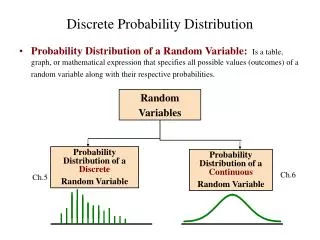
Discrete Random Variables • If the space is finite or countably infinite, a random variable X is called a discrete random variable, which maps each possible outcome of an experiment to a real number. • Pr{X=x} = {sS:X{s}=x}Pr{s} • f(x) = Pr{X=x} is the probability density function of the random variable X. • Example: • Rolling 2 dice. • X: Sum of the values on the two dice. • Pr{X=7} = Pr(1,6)+Pr(2,5)+Pr(3,4)+Pr(4,3)+Pr(5,2)+Pr(6,1) = 6/36 = 1/6. Comp 550
Expectation • Average or mean • The expected value of a discrete random variable X is E[X] = x x Pr{X=x} • Linearity of Expectation • E[X+Y] = E[X]+E[Y], for all X, Y • E[aX+Y]=aE[X]+E[Y], for constant a and all X, Y • For mutually independent random variablesX1, X2, …, Xn • E[X1X2 … Xn] = E[X1]E[X2]…E[Xn] Comp 550
Indicator Random Variables • A simple yet powerful technique for computing the expected value of a random variable. • Convenient method for converting between probabilities and expectations. • Helpful in situations in which there may be dependence. • Takes only 2 values, 1 and 0. • Indicator Random Variable for anevent Aof a sample space is defined as: Comp 550
Indicator Random Variable Lemma 5.1 Given a sample space S and an event A in the sample space S, let XA= I{A}. Then E[XA] = Pr{A}. Proof: Let Ā = S – A (Complement of A) Then, E[XA] = E[I{A}] = 1·Pr{A} + 0·Pr{Ā} = Pr{A} Comp 550
Indicator RV – Example Problem: Determine the expected number of heads in n coin flips. Method 1: Without indicator random variables. Let X be the random variable for the number of heads in n flips. Then, E[X] = k=0..nk·Pr{X=k} Comp 550
Indicator RV – Example • Method 2 : Use Indicator Random Variables • Define n indicator random variables, Xi, 1 i n. • Let Xibe the indicator random variable for the event that the ith flip results in a Head. Xi = I{the ith flip results in H} • Then X = X1 + X2 + …+ Xn = i=1..nXi. • By Lemma 5.1, E[Xi] = Pr{H} = ½, 1 i n. • Expected number of heads is E[X] = E[i=1..nXi]. • By linearity of expectation, E[i=1..nXi] = i=1..nE[Xi]. • E[X] = i=1..nE[Xi] = i=1..n½ = n/2. Comp 550
The Hiring Problem • You are using an employment agency to hire a new assistant. • The agency sends you one candidate each day. • You interview the candidate and must immediately decide whether or not to hire that person. But if you hire, you must also fire your current office assistant—even if it’s someone you have recently hired. • Cost to interview is ci per candidate. • Cost to hire isch per candidate. • You want to have, at all times, the best candidate seen so far. • When you interview a candidate who is better than your current assistant, you fire the current assistant and hire the candidate. • You will always hire the first candidate that you interview. • Problem:What is the cost of this strategy? Comp 550
Pseudo-code to Model the Scenario Hire-Assistant (n) best 0 ;;Candidate 0 is a least qualified sentinel candidate for i 1 to n do interview candidate i ifcandidate i is better than candidate best thenbest i hire candidate i • Cost Model: Slightly different from the model considered so far. • However, analytical techniques are the same. • Want to determine the total cost of hiring the best candidate. • If n candidates interviewed and m hired, then cost is nci+mch. • Have to pay nci to interview, no matter how many we hire. • So, focus on analyzing the hiring cost mch. • mch varies with order of candidates. Comp 550
Worst-case Analysis • In the worst case, we hire all n candidates. • This happens if each candidate is better than all those who came before. Candidates come in increasing order of quality. • Cost is nci+nch. • If this happens, we fire the agency. What should happen in the typical or average case? Comp 550
Probabilistic Analysis • We need a probability distribution of inputs to determine average-case behavior over all possible inputs. • For the hiring problem, we can assume that candidates come in random order. • Assign a rank rank(i), a unique integer in the range 1 to n to each candidate. • The ordered list rank(1), rank(2), …, rank(n) is a permutation of the candidate numbers 1, 2, …, n. • Let’s assume that the list of ranks is equally likely to be any one of the n! permutations. • The ranks form a uniform random permutation. • Determine the number of candidates hired on an average, assuming the ranks form a uniform random permutation. Comp 550
Randomized Algorithm • Impose a distribution on the inputs by using randomization within the algorithm. • Used when input distribution is not known, or cannot be modeled computationally. • For the hiring problem: • We are unsure if the candidates are coming in a random order. • To make sure that we see the candidates in a random order, we make the following change. • The agency sends us a list of n candidates in advance. • Each day, we randomly choose a candidate to interview. • Thus, instead of relying on the candidates being presented in a random order, we enforce it. Comp 550
Randomized Hire-Assistant Randomized-Hire-Assistant (n) Randomly permute the list of candidates best 0 ;;Candidate 0 is a least qualified dummy candidate for i 1 to n do interview candidate i ifcandidate i is better than candidate best thenbest i hire candidate i How many times do you find a new maximum? Comp 550
Analysis of the Hiring Problem (Probabilistic analysis of the deterministic algorithm) • X – RV that denotes the number of times we hire a new office assistant. • Define indicator RV’s X1, X2, …, Xn. • Xi = I{candidate i is hired}. • As in the previous example, • X = X1 + X2 + …+ Xn • Need to compute Pr{candidate i is hired}. • Pr{candidate i is hired} • i is hired only if i is better than 1, 2,…,i-1. • By assumption, candidates arrive in random order • Candidates 1, 2, …, i arrive in random order. • Each of the i candidates has an equal chance of being the best so far. • Pr{candidate i is the best so far} = 1/i. • E[Xi] = 1/i. (By Lemma 5.1) Comp 550
Analysis of the Hiring Problem • Compute E[X], the number of candidates we expect to hire. By Equation (A.7) of the sum of a harmonic series. Expected hiring cost = O(chln n). Comp 550
Analysis of the randomized hiring problem • Permutation of the input array results in a situation that is identical to that of the deterministic version. • Hence, the same analysis applies. • Expected hiring cost is hence O(chln n). Comp 550
Quicksort - Randomized Comp 550, Spring 2015
Quicksort: review Partition(A, p, r) x, i := A[r], p – 1; for j := p to r – 1 do if A[j] x then i := i + 1; A[i] A[j] fi od; A[i + 1] A[r]; return i + 1 Quicksort(A, p, r) if p < r then q := Partition(A, p, r); Quicksort(A, p, q – 1); Quicksort(A, q + 1, r) fi A[p..r] 5 A[p..q – 1] A[q+1..r] Partition 5 5 5 Comp 550
Randomized Version Want to make running time independent of input ordering. Randomized-Partition(A, p, r) i := Random(p, r); A[r] A[i]; Partition(A, p, r) Randomized-Quicksort(A, p, r) if p < r then q := Randomized-Partition(A, p, r); Randomized-Quicksort(A, p, q – 1); Randomized-Quicksort(A, q + 1, r) fi Partition(A, p, r) x, i := A[r], p – 1; for j := p to r – 1 do if A[j] x then i := i + 1; A[i] A[j] fi od; A[i + 1] A[r]; return i + 1 Comp 550
Avg. Case Analysis of Randomized Quicksort • Let RV X = number of comparisons over all calls to Partition. • Suffices to compute E[X]. Why? • Notation: • Let z1, z2, …, zn denote the list items (in sorted order). • Let RV Xij= • Thus, Xij is an indicator random variable. Xij=I{zi is compared to zj}. 1 if zi is compared to zj 0 otherwise Comp 550
Analysis (Continued) We have: Note: E[Xij] = 0·P[Xij=0] + 1·P[Xij=1] = P[Xij=1] This is a nice property of indicator RVs. (Refer to notes on Probabilistic Analysis.) So, all we need to do is to compute P[zi is compared to zj]. Comp 550
Analysis (Continued) zi and zj are compared iff the first element to be chosen as a pivot from the interval Zij is either zi or zj. Exercise: Prove this. So, Comp 550
Analysis (Continued) Substitute k = j – i. Comp 550
Algorithms Deterministic Randomized Worst-case Analysis Probabilistic Analysis Probabilistic Analysis Worst-case Running Time Average Running Time Average Running Time Deterministic vs. Randomized Algorithms • Deterministic Algorithm : Identical behavior for different runs for a given input. • Randomized Algorithm : Behavior is generally different for different runs for a given input. Comp 550
Linear Time Sort* (Ch 8 of CLRS) Z. Guo
Ch 8 of CLRS • Read Ch 8 of CLRS • There will be related HW and Exam questions • For 8.2 - 8.4, knowing “how they work” is enough. Z. Guo