James P.M. Syvitski Environmental Computation and Imaging Facility INSTAAR, CU-Boulder

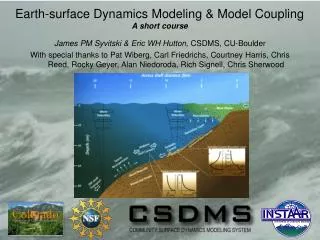
1. Earth-surface Dynamics Modeling & Model Coupling A short course James P.M. Syvitski Environmental Computation and Imaging Facility INSTAAR, CU-Boulder

2. Module 1: Process-response modeling principals ref: Syvitski, J.P.M. et al., 2007. Prediction of margin stratigraphy. In: C.A. Nittrouer, et al. (Eds.) Continental-Margin Sedimentation: From Sediment Transport to Sequence Stratigraphy. IAS Spec. Publ. No. 37: 459-530. Modelers checklist, definitions (2) From Concept to Model (6) Constraints, Sensitivity & Scaling (7) Summary (2) Earth-surface Dynamic Modeling & Model Coupling, 2009

3. Modelers checklist • Define goals of the modeling program • Outline processes to be simulated • Define assumptions behind each process and final model package • Describe conditions governing the environment being modeled: • Domain boundary conditions • Timing & location of environmental forcing: in a day, season, millennium, geologic epoch • Forcing functions: are they Periodic? Episodic? Deterministic? Probabilistic? Chaotic? • Describe the data available vs. required to meet modeling goals • Select the computational strategy and the governing equations • Select the computational schema (single vs. multi-threading) • Calibrate or verify modules • Conduct numerical experiments Earth-surface Dynamic Modeling & Model Coupling, 2009

4. Definitions SCHEMATIZATION: structure the computer uses to represent nature: discretization of space & time, boundary conditions & geometry, simplification of physical processes; i.e. how to represent wave climate or wind stress, VALIDATION: testing the applied model for compliance with nature (measurements or standards): involves calibration and verification CALIBRATION: adjustment of control parameters and boundary conditions: e.g. calibration of a 2DH tidal model with a number of water elevation and velocity data involves tuning the amplitudes and phases of the tidal constituents at the boundaries and assessing the mean water level slopes VERIFICATION: correctness of the model without further tuning or adjustment: blind test, i.e. calibration of one part of tidal cycle and prediction for the other. BENCHMARKING: Measure (speed, accuracy) of one model against another, given constrained inputs and boundary conditions Earth-surface Dynamic Modeling & Model Coupling, 2009

5. FROM CONCEPT TO MODEL Earth-surface Dynamic Modeling & Model Coupling, 2009

6. Statistical model:relationships amongst simultaneously-varying attributes are analyzed. Relationships not previously recognized may be indicated. Empirical model:variables interrelated in a predictive algorithm. e.g. polynomial model to estimate the transport of suspended sediment to the ocean: variables include discharge, suspended sediment concentrations -based on observations and limited to environments with similar conditions Response model loop: (1) predictions are made (2) new observations collected to test predictive model (3) conceptual model revised (4) statistical testing and generation of refined empirical model Earth-surface Dynamic Modeling & Model Coupling, 2009

7. The Process Model: e.g. based on fundamental theory. • theoretical expressions of physical or biophysical laws (e.g. fluid mechanics), considered mathematical approximations of reality, that when linked together can describe a physical system. • include conservation equations of mass, momentum, and energy. • continuity equations keep track of volume or mass within the system being modeled: e.g. Exner (erosion – deposition) • conservation of energy equation e.g. conversion of turbulence to work done (erosion, suspension) • conservation of momentum equation: operating forces at a given location and boundary shear stresses. • some parameters are determined fairly accurately and others are merely constrained estimates. • untested theory is the weak link in a model Earth-surface Dynamic Modeling & Model Coupling, 2009

8. Advection- Diffusion ∂x Navier-Stokes Momentum Navier-Stokes Energy Parker & Imran et al., formulation of the debris flow momentum Earth-surface Dynamic Modeling & Model Coupling, 2009

9. Numerical Simulation: • Methods: finite difference (localized approximations) versus finite element (global constraints of the full domain). • Solutions (explicit schemes, implicit schemes and method of characteristics) depend on form of the differential equation (elliptic, parabolic, or hyperbolic). Earth-surface Dynamic Modeling & Model Coupling, 2009

10. Data Assimilation & Predictive Modeling Temperature, Winds Tides, Waves Heat & Momentum Flux Precipitation, Temperature, Winds River, Sediment Discharge Earth-surface Dynamic Modeling & Model Coupling, 2009

11. CONSTRAINTS TO A PROCESS-RESPONSE MODEL • Principles of hydrodynamics must be observed. • e.g. critical stress governing the deposition of a particle from suspension must be less than the critical stress governing the erosion from the sea floor of that same particle • (2) Laws of conservation must be adhered to • e.g. often governing equations can only be approximated … numerical transport algorithms can lead to artificial diffusion when properties are considered constant throughout the cell • (3) Boundary conditions must be realistic and not contribute to instabilities. • e.g. A diffusion equation relates bulk transport to concavity of the slope. Critical boundary state occurs when all sediment is removed by diffusion and rock basement is encountered. • (4) Use realistic inputs from the external world, i.e. outside the immediate area • e.g. tides in the Bay of Fundy, the area where sediment transport was to be predicted, is based on a numerical grid that included the entire Gulf of Maine, an area nearly two orders-of-magnitude larger. Earth-surface Dynamic Modeling & Model Coupling, 2009

12. SENSITIVITY ANALYSIS • used to determine the importance of various parameters in affecting the final result of a model's algorithms. • allows the modeler to test both numerical stability and validity in boundary conditions, by choosing extreme values of input. • a parameters sensitivity depends on the magnitude of its exponential and the range of its variability • complex models often have many convoluted interactions that computer simulations are the only means to ascertain the sensitivity of a particular parameter. Earth-surface Dynamic Modeling & Model Coupling, 2009

13. SCALING TIME Wiberg, UVA 12 x 105 Suspended Load of the Po River during LGM 8 x 105 Year 1 Year 2 4 x 105 Scaling the cross-shelf sediment flux using various wave forcing averages Cross shelf Distance (km) Low Frequency, High Magnitude Events (PDF-CDF approach) Hutton/Syvitski, INSTAAR • Scaling Analysis: • Scaling Time; • Scaling Space; • Scaling Dynamics; • Scaling Variability; • Upscaling; • Downscaling Earth-surface Dynamic Modeling & Model Coupling, 2009

14. SCALING TIME 16 300 12 16 frequency 200 12 frequency frequency 8 Yearly time steps 8 100 Daily time steps 4 4 0 0 1 2 3 4 0 1 2 3 4 Wave Height (m) Wave Height (m) frequency Yearly time steps Daily time steps 160 0 10 20 30 40 0 10 20 30 40 Wavelength (m) Wavelength (m) 120 80 40 0 Experiments with Time Steps Daily Time Step Yearly Time Step Hutton/Syvitski INSTAAR For long time steps, only model the large events Earth-surface Dynamic Modeling & Model Coupling, 2009

15. Scaling Variability Experiments on Wave Variability High Wave Variability Low Wave Variability 20km core 30km core 20km core 30km core Examples of erosion surfaces from major storms Wave heights 2.1±1m Wavelengths 21±10m Wave heights 2.1±0.1m Wavelengths 21±1m Earth-surface Dynamic Modeling & Model Coupling, 2009

16. Scaling Dynamics Resuspended sediment volume per day as a function of wave height Final profiles of modeled bathymetry Scaling reduces run time by 75%. Earth-surface Dynamic Modeling & Model Coupling, 2009

17. Resolution Earth-surface Dynamic Modeling & Model Coupling, 2009

18. Earth-surface Dynamic Modeling & Model Coupling, 2009

19. Process-Response Modeling should push scientists to confront nature • is one process coupled or uncoupled to another • is a particular process deterministic or stochastic • level of simplification (1D, 2D, 3D) • has an analytical solution for a particular process been formulated yet • how are processes scaled across time and space • adequacy of databases on key parameters from field or laboratory measurements Earth-surface Dynamic Modeling & Model Coupling, 2009