Download
1 / 47
470 likes | 609 Vues
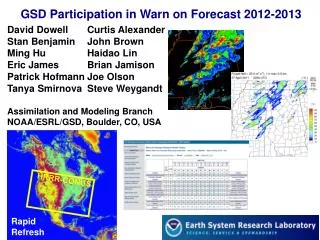
GSD Participation in Warn on Forecast 2012-2013. David Dowell Curtis Alexander Stan Benjamin John Brown Ming Hu Haidao Lin Eric James Brian Jamison Patrick Hofmann Joe Olson Tanya Smirnova Steve Weygandt Assimilation and Modeling Branch NOAA/ESRL/GSD, Boulder, CO, USA. HRRR-CONUS. Rapid

E N D
GSD Participation in Warn on Forecast 2012-2013 David Dowell Curtis AlexanderStan Benjamin John Brown Ming Hu Haidao Lin Eric James Brian Jamison Patrick Hofmann Joe Olson Tanya Smirnova Steve WeygandtAssimilation and Modeling BranchNOAA/ESRL/GSD, Boulder, CO, USA HRRR-CONUS Rapid Refresh
Outline • Case Studies: Storm-Scale Radar-Data Assimilation and Ensemble Forecasting • 27 April 2011 • VORTEX2 cases • Website Development to Enhance Collaboration • Real-Time, Hourly-Updated Model Development • candidates for nested WoF systems • RAP and HRRR • NARRE and HRRRE • 2013 Priorities / Wish List
27 April 2011 SupercellTornado Outbreak Retrospective Storm-Scale Ensemble Radar DA and Forecasting: Goals • Test drive “state-of-the art” radar DA methods for a large number and variety of retrospective cases • Examine forecast ensemble spread resulting from storm-scale perturbations (and other sources) for real cases • complementary to OSSE work by Corey Potvin • ensemble sensitivity analysis Tuscaloosa, AL tornado source: CBS 42 Birmingham, AL
Experiment Summary: 4/27/2011 Tornado Outbreak • 45-member ARW ensembles (Dx=3 km) initialized from NAM and RAP • 600-km domain for these preliminary experiments • Velocity and reflectivity data assimilated every 3 min for 1 h • KBMX, KDGX, KGWX, KHTX ; simple, automated quality control • additive storm-scale pert. during cycled radar DA -- only source of ensemble spread • WRF-DART ensemble adjustment Kalman filter • Ensemble forecast produced after radar DA ensemble experiments KHTX 19Z 20Z 21Z 22Z 23Z 0Z NAM/ RAP init. KGWX radar DA ensemble forecast KBMX KDGX control experiments 19Z 20Z 21Z 22Z 23Z 0Z NAM/ RAP init. deterministic forecast
Probability of Rotating Updrafts (2-5 km updraft helicity > 25 m2 s-2) 2000-2100 UTC NSSL Composite Reflectivity 2000 UTC 500 km control experiment (no radar DA, deterministic forecast) radar DA, 0-1 h ensemble forecast 2100 UTC
Probability of Rotating Updrafts (2-5 km updraft helicity > 25 m2 s-2) 2000-2100 UTC NSSL Composite Reflectivity 2000 UTC 500 km control experiment (no radar DA, deterministic forecast) radar DA, 0-1 h ensemble forecast 2100 UTC removing spurious storms from analysis and forecast still a challenge for radar DA
Probability of Rotating Updrafts (2-5 km updraft helicity > 25 m2 s-2) 2000-2100 UTC NSSL Composite Reflectivity 2000 UTC 500 km control experiment (no radar DA, deterministic forecast) radar DA, 0-1 h ensemble forecast 2100 UTC radar DA reorganizes storms in region where mesoscale environment (observed and simulated) was already supportive of convective storms
Probability of Rotating Updrafts (2-5 km updraft helicity > 25 m2 s-2) 2000-2100 UTC NSSL Composite Reflectivity 2000 UTC 500 km control experiment (no radar DA, deterministic forecast) radar DA, 0-1 h ensemble forecast 2100 UTC radar DA introduces viable storms where they were needed; (CI enhanced through radar DA, maintenance supported by mesoscale environment in model)
Probability of Rotating Updrafts (2-5 km updraft helicity > 25 m2 s-2) 2000-2100 UTC NSSL Composite Reflectivity 2100 UTC 500 km control experiment (no radar DA, deterministic forecast) radar DA, 1-2 h ensemble forecast 2200 UTC some storms introduced by radar DA persist; probabilities vary among storms
Ensemble Forecast (105 min) Composite Reflectivity Spread Mean NSSL Composite Reflectivity 2145 UTC
Ensemble Forecast (105 min) Composite Reflectivity Spread Mean southern storm: high mean, low spread NSSL Composite Reflectivity 2145 UTC
Ensemble Forecast (105 min) Composite Reflectivity Spread Mean southern storm: high mean, low spread northern storm: low mean, high spread NSSL Composite Reflectivity 2145 UTC
Ensemble Sensitivity Analysis (work in progress) Spread Mean • ensemble-based correlations between initial conditions (and/or model parameters) and forecast metric • method applied previously to larger scales (Hakim and Torn 2008) • ongoing work to apply to convective scale • What types of storm-scale perturbations resulted in the northern storm persisting in the forecast?
VORTEX2 Case Studies • 18 May 2010 Dumas, Texas Supercell • collaboration with Texas Tech University (Chris Weiss, Tony Reinhart, Pat Skinner) • 5 June 2009 Goshen County, Wyoming Supercell • collaboration with Penn State University (Jim Marquis et al.) • foci: assimilation of radar and surface observations into high- • resolution models, diagnosis of severe storm processes photo by David Dowell for VORTEX2
18 May 2010 Dumas, TX Storm: Observations and Analysis KAMA verification of surface fields StickNet DOW6 DOW7 SR1 KAMA assimilation of KAMA, SR1, DOW6, and DOW7 data
, lowest model level StickNet 80 km
Perturbation* Temperature (K) 2300 UTC StickNet (circles) and Ensemble Mean (outside circles) * relative to model’s base state 2 m AGL (StickNet) 8 m AGL (simulation) 2 K contour interval 10 km
Perturbation* Temperature (K) 2344 UTC StickNet (circles) and Ensemble Mean (outside circles) * relative to model’s base state 2 m AGL (StickNet) 8 m AGL (simulation) 2 K contour interval 10 km
Westerly (u) Wind Component 2328 UTC StickNet (circles) and Ensemble Mean (outside circles) 2 m AGL (StickNet) 8 m AGL (simulation) 3 m s-1 contour interval 10 km
Web Graphics for Warn-on-Forecast Experiments WRF NetCDF tool for enhancing our collaboration, leveraging community software and scripts developed previously for RAP-HRRR (acknowledgments: Brian Jamison, Susan Sahm) quick, easy sharing of results from retrospective and real-time experiments rough drafts of websites: rapidrefresh.noaa.gov/WoFMeso/ rapidrefresh.noaa.gov/WoFSS/ Unipost GRIB2 NCL .png web display
Hourly-Updated NOAA NWP Models 13km Rapid Refresh • Rapid Refresh • High-Resolution Rapid Refresh • NARRE • hourly-updated ensemble, 10-12 km, hybrid/EnKF DA • 2015-2016? • HRRRE • hourly-updated ensemble, 3 km • 2017-2018? • All are candidate models for nested WoF systems. 3km HRRR
HRRR Verification 2011 vs 2012 Eastern US, Reflectivity > 25 dBZ 11-21 August 2011 40 km CSI ( x 100) 13 km bias (x 100) 2011 HRRR 2012 HRRR Optimal MUCH reduced bias for HRRR 2012, similar CSI
2013: Cycled Reflectivity at 3 km 13 km RAP 13z 14z 15z Obs Obs Obs GSI 3D-VAR GSI 3D-VAR GSI 3D-VAR HM Obs HM Obs HM Obs Cloud Anx Cloud Anx Cloud Anx 1 hr fcst 1 hr fcst Refl Obs Refl Obs Refl Obs Digital Filter Digital Filter Digital Filter 18 hr fcst 18 hr fcst 18 hr fcst 3-km Interp 3 km HRRR 15 hr fcst 1 hr pre-fcst 1-hr Reduction In Latency for 14z HRRR 3-km Interp Refl Obs
Additional Positive Contribution to HRRR (3-km) Forecasts from Reflectivity DA in HRRR Critical Success Index (CSI) for 25-dBZ Composite Reflectivity reflectivity DA in RAP + HRRR (for 1 h) reflectivity DA in RAP only upscaled to 40-km grid 14-day June 2011 retrospective period verification over eastern half of US (widespread convective storms)
Time-lagged ensemble Model Init Time Example: 13z + 2, 4, 6 hour HTPF Model runs used 18z 17z 16z 15z 14z 13z 12z 11z 13z+2 12z+3 11z+4 13z+4 12z+5 11z+6 13z+6 12z+7 11z+8 model has 2hr latency HTPF 2 4 6 11z 12z 13z 14z 15z 16z 17z 18z 19z 20z 21z 22z 23z Forecast Valid Time (UTC)
The HCPF and HTPF HRRR Convective Probabilistic Forecast (HCPF) HRRR Tornadic Storm Probabilistic Forecast (HTPF) Use time-lagged ensemble to estimate liklihood of convection and tornado production Identification of updraft rotation using model forecast fields: • Intensity – Maximum Updraft Helicity 2-5 km AGL ≥ 25 m2 s-2 • Time – Two hour search window centered on valid times • Location – Searches within 45 km (15 gridpoints) of each point for each member • Members – Three consecutive HRRR initializations HTPF = # grid points matching criteria over all members total # grid points searched over all members
Example: 27 April 2011 13z + 09hr fcst Valid 22z 27 April 2011 Observed Reflectivity 22z 27 April 27 April 2011 Storm Reports Valid 1200-1200 UTC 28 Apr Tornadic Storm Probability (%) Reflectivity (dBZ) Tornado = Red Dots
Priorities / Wish List for 2013 • National quality-controlled WSR-88D datasets – including Doppler velocity – for retrospective and real-time radar DA experiments • nonmeteorological data removal utilizing polarimetric information • Collaboration on regional storm-scale radar DA and ensemble forecasting for retrospective periods ~1 week • parameter space: multiple radar DA methods, multiple resolutions, … • common radar observations for input, model configuration, forecast verification • 3-km ensemble for background
RAP and HRRR Model Details HRRR RAP diabatic digital filter initialization with radar-reflectivity and lightning (proxy refl.) data observations assimilated with GSI (3DVar) into experimental RAP at ESRL rawinsonde; profiler; VAD; level-2.5 Doppler velocity; PBL profiler/RASS; aircraft wind, temp, RH; METAR; buoy/ship; GOES cloud winds and cloud-top pres; GPS precip water; mesonet temp, dpt, wind (fall 2012); METAR-cloud-vis-wx; AMSU-A/B/HIRS/etc. radiances; GOES radiances (fall 2012); nacelle/tower/sodar
Positive Contribution to HRRR (3-km) Forecasts from Reflectivity DA (DDFI) in Parent (13-km) RAP Critical Success Index (CSI) for 25-dBZ Composite Reflectivity HRRR with RAP reflectivity DA (real time) HRRR without RAP reflectivity DA upscaled to 40-km grid 11-20 August 2011 retrospective period verification over eastern half of US (widespread convective storms)
Latent Heating (LH) Specification Temperature Tendency (i.e. LH) = f(Observed Reflectivity) LH specified from reflectivity obs applied in four 15-min periods The observations are valid at the end of each 15-min pre-fcst period NO digital filtering at 3-km Hour old mesoscale obs Latency reduced by 1 hr -60 -45 -30 -15 0 Observed 3-D Radar Reflectivity Time (min) LH = Latent Heating Rate (K/s) p = Pressure Lv = Latent heat of vaporization Lf = Latent heat of fusion Rd = Dry gas constant cp = Specific heat of dry air at constant p f[Ze] = Reflectivity factor converted to rain/snow condensate t = Time period of condensate formation (600s i.e. 10 min) -60 -45 -30 -15 0 Model Pre-Forecast Time (min)
Diabatic Digital Filter Initialization (DDFI) -20 min -10 min Init +10 min Backward integration, no physics Forward integration, full physics Apply latent heating from radar reflectivity, lightning data Obtain initial fields with improved balance, vertical circulations associated with ongoing convection RR model forecast The model microphysics temperature tendency is replaced with a reflectivity-based temperature tendency. Dynamics respond to forcing. Analysis noise is reduced by digital filtering.
Anticipated Progression of RAP and HRRR Radar DA radar data obs 3DVar + cloud analysis DDFI RAP 13 km … … fcst fcst t02 h t01 h t0 interpolation HRRR 3 km fcst radar data radar data radar data radar data • now: radar DA in RAP (13 km) only • near future (proposed): continued radar DA in RAP (13 km); • short period of radar DA in HRRR (3 km) before HRRR forecast begins • future: cycling with all obs (including radar) on HRRR (3-km) grid • 3DVar and reflectivity-based temperature tendency • hybrid / ensemble DA and forecasting • HRRR reflectivity DA • same formulation of reflectivity-based temperature tendency as in RAP • no digital filter
radar data obs 3DVar + cloud analysis DDFI RAP 13 km … … fcst fcst t02 h t01 h t0 interpolation HRRR 3 km fcst radar data obs 3DVar + cloud analysis DDFI RAP 13 km … … fcst fcst t02 h t01 h t0 interpolation HRRR 3 km fcst radar data radar data radar data radar data ExperimentComparison (1) HRRRinitialized“without 3-kmradar DA” (2) HRRRinitialized“with 3-kmradar DA”
CompositeReflectivity2300 UTC11 June 2011 observations mature convective systems benefit particularly from subhourly radar DA 1-h fcstwithout 3-kmradar DA 1-h fcstwith 3-kmradar DA 1000 km
Model and Data Assimilation • WRF model run as “cloud model” • homogeneous base state; no parameterizations for PBL, surface layer, radiation, … • Dx = 1000 m, Dz = 50 to 500 m • Lin et al. (1983) precipitation microphysics, configured for hail and large raindrops • n0(hail) = 4 × 10⁴ m-4 n0(rain) = 1 × 10⁶ m-4 • weaker cold pool (Gilmore et al. 2004) than for default scheme, but still strong… • Radar data assimilated every 2 min for 3 hours • Data Assimilation Research Testbed (DART) ensemble Kalman filter • KAMA reflectivity and Doppler velocity throughout period • mobile Doppler velocity (SR1, DOW6, DOW7) when available • 60-member ensemble • variability from (1) random perturbations to base-state wind profile and (2) random • local perturbations to horizontal wind, temperature, and humidity (dewpoint) • “analysis” (“simulation”) is prior ensemble mean • Verification of model surface fields with StickNet observations • first, determine if the model is capable of simulating the storm and environmental • features of interest in radar-DA-only experiments • later, assimilate surface (StickNet and MM) observations into “final” analysis
Westerly (u) Wind Component 2314 UTC StickNet (circles) and Ensemble Mean (outside circles) 2 m AGL (StickNet) 8 m AGL (simulation) 3 m s-1 contour interval 10 km
Summary of Surface Verification Overall patterns are reasonable; differences involve the details. Cooling in the downshear precipitation core is too weak in the simulation. consistent with perceived errors in single-moment microphysics schemes The main body of the simulated cold pool is generally too cold and too widespread. consistent with perceived errors in single-moment microphysics schemes StickNet winds (2 m AGL) are generally weaker than model winds (8 m AGL). implications for diagnosis of “baroclinic”, “barotropic”, and “friction- induced” contributions to mesocyclone rotation model lower boundary condition currently free slip; more realistic surface and boundary layer needed for simulation and data assimilation
Challenges of Storm-Scale DA and NWP • Large radar datasets in need of quality control • Large model grids • 1000’s of km wide, grid spacing ~1 km • Model error and predictability • unresolved processes: updraft, downdraft, precipitation microphysics, PBL, … • predictability time scale ~10 min for an individual thunderstorm • forecast sensitivity to small changes in initial conditions (e.g., water vapor) • Flow-dependent background-error covariances • no quasi-geostrophic balance on small scales • retrieving unobserved fields • Verifying forecasts (to improve future ones) • unobserved fields, isolated phenomena • All tasks (preprocessing and assimilating obs, producing forecasts) must occur quickly for the forecast to be useful in real time! • within an hour for some applications • within minutes for warning guidance 190 radars volumes every 10 min or less