Fixed parameter tractability and kernelization for the Maximum Leaf Weight Spanning Tree problem

1. Bart Jansen, Utrecht University Fixed parameter tractability and kernelization for the Maximum Leaf Weight Spanning Tree problem

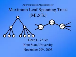
2. Maximum Leaf Spanning Tree • Max Leaf • Instance: Connected graph G, positive integer k • Question: Is there a spanning tree for G with at least k leaves? • Applications in network design • YES-instance for k ≤ 7

3. Complexity of Max Leaf • Classicalcomplexity • MAX-SNP complete, sonopolynomial-timeapproximationscheme (PTAS) • NP-complete, even for

4. BipartiteMax Leaf Spanning Tree • Bipartite Max Leaf • Instance: Connectedbipartitegraph G withblack and whiteverticesaccording to the partition, positive integer k • Question: Is there a spanning tree for G with at least k blackleaves?

5. Complexity of Bipartite Max Leaf • Classicalcomplexity • No constant-factorapproximation • NP-complete, even for:

6. Max LeafWeight Spanning Tree • Weighted Max Leaf • Instance: Connected graph G with a non-negative integer weight for each vertex, positive integer k • Question: Is there a spanning tree for G such that its leaves have combined weight at least k? Leafweight 11 Leafweight 16

7. Complexity of Weighted Max Leaf • Classical complexity • NP-complete by restriction of the previous problems • Hard on all classes of graphs mentioned so far • No constant-factor approximation since it generalizes Bipartite Max Leaf • We consider the fixed parameter complexity

8. Fixed parameter complexity • Technique to deal with problems (presumably) not in P • Asks if the exponential explosion of the running time can be restricted to a “parameter” that measures some characteristic of the instance • An instance of a parameterized problem is: • <I,k> where k is the parameter of the problem (often integer) • Class of Fixed Parameter Tractable (FPT) problems: • Decision problems that can be solved in f(k) * poly(|I| + k) time • Function f can be arbitrary, so dependency on k may be exponential • For example, the k-Vertex Cover problem is fixed parameter tractable. • “Is there a vertex cover of size k?” • Can be solved in O(n + 2k k2) (and even faster).

9. Kernelization algorithms • A kernelization algorithm: • Reduces parameterized instance <I,k> to equivalent <I’,k’> • Size of I’ does not depend on I but only on k • Time is poly (|I| + k) • New parameter k’ is at most k • If |I’| is O(g(k)), then g is the size of the kernel • Kernelization algorithm implies fixed parameter tractability • Compute a kernel, analyze it by brute force

10. Fixed parameter (in)tractability • Existing problems, parameterized by nr. of leaves • Regular Max Leaf has a 3.5k kernel • No FPT results for Bipartite Max Leaf • For Weighted Max Leaf • We take the target weight k as the parameter of the problem • (In)tractabledependingonwhetherweight 0 is allowed • Kernelsizedependsonclass of graphs

11. Fixed parameter intractability Bipartite Max Leaf is hard for W[1]

12. Parameterized complexity classes • Unless the Exponential Time Hypothesis is false, being W[1] hard implies: • No f(k)*p(n) algorithm • No polynomial-size kernel • W[2]-hard is assumed to be harder than W[1]-hard • For Weighted Max Leaf: • No proof of membership in W[1] • It might be harder than any problem in W[1] • No hardness proof for W[2] either

13. Reductions prove W[1] hardness • W[i] hardness is proven by parameterized reduction <I,k>  <I’,k’> from some W[i]-hard problem • Like (Karp) reductions for NP-completeness • Extra condition: new parameter k’ ≤ f(k) for some f • We reduce k-Independent Set (W[1]-complete) to Bipartite Max Leaf

14. Setup for reduction • k-Independent Set • Instance: Graph G, positive integer k • Question: Does G have an independent set of size at least k? • (i.e. is there a vertex set S of size at least k, such that no vertices in S are connected by an edge in G?) • Parameter: the value k.

15. Reduction from k-Independent Set • Given an instance of k-Independent Set, we reduce as follows: • Color all vertices black • Split all edges by a white vertex • Add white vertex w with edges to all black vertices • Set k’ = k • Polynomial time • k’ ≤ f(k) = k

16. Leaves and cutsets • If S is a cutset, then at least one vertex of S is internal in a spanning tree • We need to give at least one vertex in S a degree ≥ 2 to connect both sides

17. Independent set of size k  Spanning tree with ≥ k black leaves • Complement of S is a vertex cover • Build spanning tree: • Take w as root, connect to all blacks • We reach the white verticesfrom the vertex cover V – S • Sinceevery white vertexused to beanedge Edges incident on w are not drawn

18. Spanning tree with k black leaves  Independent set of size k • Take the black leaves as the independent set • Ifthere was anedge x,y thenthey are notbothleaves • Since {x,y} is a cutset • Bycontraposition, black leavesforman independent set Edges incident on w are not drawn

19. Fixed parameter tractability A linear kernel for Maximum Leaf Weight Spanning Tree on planar graphs

20. A linearkernelforWeighted Max Leafonplanargraphs • Kernel of size 84k on planar graphs • Strategy: • Give reduction rules • that can be applied in polynomial time • that reduce the instance to an equivalent instance • Prove that after exhaustive application of the rules, either: • the size of the graph is bounded by 84k • or we are sure that the answer is yes • then we output a trivial, constant-sized YES-instance

21. Kernelization lemma • We want to be sure that the answer is YES if the graph is still big after applying reduction rules • Use a lemma of the following form: • If no reduction rules apply, there is a spanning tree with |G|/c leaves of weight ≥ 1 (for some c > 0) • With such a proof, we obtain: • If |G| ≥ ck then G has a spanning tree with |G|/c≥ck/c=k leaves of weight 1 • So a spanning tree with leaf weight ≥ k • So if |G| ≥ ck after kernelization we return YES • Otherwise the instance must be small

22. The reduction rules • The reduction rules must avoid the following situation: • We can build an arbitrarily large graph with only constant leaf weight in an optimal spanning tree • All reduction rules are needed to prevent such situations • Reduction rules are motivated by examples of the situations they prevent

23. Terminology • A set S of vertices is a cutset if their removal splits the graph into multiple connected components • A path component of length k is a path <x,v1,v2, .. , vk,y>, s.t. • x, y have degree ≠ 2 • all vi have degree 2

24. Bad situation 1) • Vertex of positive weight, with arbitrarily many degree-1 neighbors of weight 0

25. 1) Removedegree 1 vertices • Structure: • Vertex x of degree 1 adjacent to y of degree > 1 • Operation: • Delete x, decrease k by w(x), set w(y) = 0 • Justification: • Vertex x will be a leaf in any spanning tree • The set {y} is a cutset, so y will never be a leaf in a spanning tree k’ = k – w(x)

26. Bad situation 2) • A connected component of arbitrarily many vertices of weight 0

27. 2) Contract edgesbetween weight-0 vertices • Structure: • Two adjacent weight-0 vertices x, y • Operation: • Contract the edge xy, let w be the merged vertex • Justification: • Tree T  Tree T’: • There always is an optimal tree that uses xy • Addxy to tree, removeanedgefromresultingcycle • Verticesxy have weight 0 sono loss of leafweight • Contract the edgexy to obtain T’ • Tree T’  Tree T: • Split w intotwovertices x, y and connect to neighbors

28. Bad situation 3) • Arbitrarily many weight-0 degree-2 vertices with the same neighborhood

29. 3) Duplicate degree-2 weight-0 vertices • Structure: • Two weight-0 degree-2 vertices u,v with equal neighborhoods {x,y} • The remainder of the graph R is not empty • Operation: • Remove v and its incident edges • Justification: • {x, y} forms a cutset • One of x,y will always be internal in a spanning tree

30. Bad situation 4) • A necklace of arbitrary length • Every pair of positive-weight vertices forms a cutset, so at most 1 leaf of positive weight

31. 4) Edgebypassing a weight-0 vertex • Structure: • a weight-0 degree-2 vertex with neighbors x,y • a direct edge xy • Operation: • remove the edge xy • Justification: • You never need xy • If xy is used, we might as well remove it and connect x and y through z • Since w(z) = 0, leaf weight does not decrease

32. Bad situation 5) • Three path components of arbitrary length • At most 4 leaves in any spanning tree

33. 5) Shrinklargepathcomponents • Structure: • Path component <x,v1,v2,..,vp,y> with p ≥ 4 • Operation: • Replace v2,v3, .. , vp-1 by new vertex v* • Weight of v* is maximum of edge endpoints – max(w(v1),w(vp)) • Justification: • The two spanning trees are equivalent • If a spanning tree avoids an edge inside the path component, then the optimal leaf weight gained is equal to the leaf weight gained by avoiding an edge incident on v*

34. Bad situation 6) • An arbitrarily long cycle with alternating weighted / zero weight vertices • At most one leaf of positive weight

35. 6) Cut a simplecycle • Structure: • The graph is a simple cycle • Operation: • Remove an edge that maximizes the combined weight of its endpoints • Justification: • Any spanning tree for G avoidsexactlyoneedge • Avoidinganedgewith maximum weight of endpoints is optimal

36. About the reduction rules • These reduction rules are necessary and sufficient for the kernelization claim • Reduction rules do not depend on parameter k • Reduced instance is the same, regardless of k • Reduction rules do not depend on planarity of the graph • But the structural proof that every reduced instance has a |G|/c leaf weight spanning tree does depend on k • Reduction rules can be executed in linear time • Planarity is preserved • We only remove and contract edges • Suggests the reduction rules are good preprocessing rules for any instance of Weighted Max Leaf • Even non-planar graphs without given parameter • The structural proof is constructive • When the output of kernelization is YES then we can also find a suitable spanning tree

37. Structure of a reduced instance • We apply the reduction rules in the given order, until no rule is applicable • Can be done in linear time • Reduced graph is still planar, since all we do is: • Contract an edge, remove an edge, remove a vertex, re-color a vertex. • Reduced instance is highly structured: • White vertices form an independent set • All vertices have degree ≥ 2 • No path components of size > 3 • …

38. FPT algorithm using kernelization • Kernelization yields FPT algorithm • First kernelize, then try all possible leaf sets • Check whether the complement is a connected dominating set • Planar graphs are sparse, so |E| is O(|V|) • Kernelization can be implemented to run in linear time

39. Summary • Maximum Leaf Weight Spanning tree is a natural generalization of the Maximum Leaf Spanning Tree problem • It is W[1]-hard on general graphs, so no FPT algorithm • The problem admits a 84k problem kernel on planar graphs • This can be extended to: • O(k √g) kernelongraphs of genus g • O(k d) kernel on graphs on which every vertex of positive weight has at most d neighbors

40. Future work • Decreasing constant in the kernel size • Better mathematical analysis of resulting reduced instances • New reduction rules needed to go below 24k kernel • Classifying complexity of general-graph problem • Hardness proof for some W[i] > 1 • Membership proof for some W[i] • Determining complexity for real-valued weights • Approximation algorithms • Does (Weighted) Max Leaf have a PTAS onplanargraphs?