Unit 3 Summary Statistics (Descriptive Statistics) FPP Chapter 4
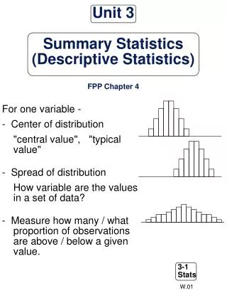
For one variable - - Center of distribution "central value", "typical value" - Spread of distribution How variable are the values in a set of data? - Measure how many / what proportion of observations are above / below a given value.

Unit 3 Summary Statistics (Descriptive Statistics) FPP Chapter 4
E N D
Presentation Transcript
For one variable - - Center of distribution "central value", "typical value" - Spread of distribution How variable are the values in a set of data? - Measure how many / what proportion of observations are above / below a given value. Unit 3Summary Statistics(Descriptive Statistics)FPP Chapter 4 W.01
We will discuss: • how the statistics are defined • when each is (in)appropriate • how to interpret them • how to compute them • "guesstimation" techniques Summary Statistics Purposes: compact reporting easy comparison Important considerations: interpretable stable
Total charge (in dollars) of the hospital stay for 29 normal deliveries of babies Example: Hospital Charges Charges 1,905 2,324 2,048 2,888 2,907 2,840 2,607 2,823 2,310 2,953 2,138 3,418 4,903 3,729 3,709 5,063 3,932 3,392 3,287 3,819 4,248 2,640 2,921 2,785 2,804 2,955 2,219 2,184 2,681 14,898
12 Definitions 10 8 freq. 6 4 2 1500 2500 3500 4500 5500 Hospital Charges (in Dollars) mode = most frequently occurring value = _______________ median = "middle value" = __________________ = mean = sum / # measurements in the data set = = __________/___________ = _________ = another way to compute the mean:
mode: median: mean: comparing mean & median: For skewed histograms, the mean could be deceiving. Locating These SummaryStatistics on a Histogram 12 10 8 freq. 6 4 2 1500 2500 3500 4500 5500 Hospital Charges (in Dollars)
(ref. "Marketing Science", Fall 1987, vol 6, no 4, pages 320-335, "Does It Pay to Change Your Company's Name?") -1.84 -0.31 0.02 0.30 0.53 1.09 -1.38 -0.24 0.06 0.34 0.55 1.12 -1.00 -0.24 0.09 0.36 0.58 1.23 -0.59 -0.20 0.10 0.39 0.78 1.43 -0.57 -0.16 0.13 0.40 0.81 1.50 -0.56 -0.06 0.21 0.41 0.96 1.60 -0.51 -0.05 0.23 0.43 0.98 1.64 -0.44 -0.02 0.24 0.45 0.99 1.79 -0.39 -0.02 0.25 0.48 1.00 -0.33 -0.01 0.29 0.50 1.03 Event Day Abnormal Returns
mode = most frequently occurring value =______ median = "middle value" = __________ mean = "average" = (sum of values in list)/(# values in list) = _____ / _____ = _____ p th percentile = the value with p percent of the list less than (or equal to it) and 100-p percent greater than it 10 th percentile = _____ 25 th percentile = _____ 80 th percentile = _____
Histogram for Abnormal Returns 0.4 20 0.3 15 0.2 10 0.1 5 -2.0 -0.5 1.0 2.5 4.0 RETURNS
Some summary statistics make sense only for certain types of data. mean: median: mode: Does This Statistic Make Sense?
Aug 1-22 the average consumption was 223.7 million gallons per day. Aug 1-25 the average consumption was 224.4 million gallons per day. Q1: Was the average consumption higher Aug 1-22 or Aug 23-25? Q2: What was the total amount of water consumed Aug 23-25? Q3: What was the average daily consumption Aug 23-25?
Suppose batting average = (# hits / # at bats) x 1000 Before the game starts, a player has batting average = 250. - first at bat, strikes out - new batting average = 200 Q1: How many times has this batter been up? Another player starts the game with batting average 500. After his first at bat, his new batting average is 524. Q2: Did he get a hit? Q3: How many times has this batter been up? Baseball Batting Averages
LOCATION mean median mode SPREAD standard deviation (SD) range variance Measures ofLocation & Spreadof a Data Set
RANGE: (largest measurement) - (smallest measurement) example: Range
definition: deviation from average = data value - average note: A deviation can be zero. 1 2 5 7 10 data value Deviation from Average
definition: standard deviation = SD = rms size of the deviations from average = Standard Deviationof a list of numbers
root-mean-square (rms) operation 1 2 5 7 10 data value deviation rms (root mean square) size of a list of numbers
Find the standard deviation (rms size of the deviations from average) for this list of numbers. 2, - 6, 12, 4, 6 I. Find the average of this list of numbers. II. Find the deviation of each value from this average. III. Find the rms size of the list of deviations. -6 -5 -4 -3 -2 -1 0 1 2 3 4 5 6 7 8 9 10 11 12 data Standard Deviation Try another list of numbers.
The STANDARD DEVIATION (SD) OF A DATA SET measures how far away numbers are from their average. Most entries on the list will be somewhere around one SD away from the average. Very few will be more than two or three SDs away. Standard Deviation
* Roughly 68% of the entries on a list (roughly 2/3 of the entries) are within one SD of the average. * The other 32% (approximately 1/3) are further away. ** Roughly 95% (19 out of 20) are within two SDs of the average. ** The other 5% are further away. The 2/3 rule is true for most data sets. The 95% rule is true for many data sets, but not all. Interpreting theStandard Deviation
Class LimitsTallies Frequency 25-34 | 1 35-44 ||| 3 45-54 |||| 4 55-64 | 1 65-74 |||| ||| 8 75-84 |||| |||| 10 85-94 |||| |||| 9 95-104 ||| 3 105-114 |||| 4 115-124 |||| 5 125-134 || 2 Delivery Times Example TIME IN DAYS 27 68 79 91 107 43 71 80 91 108 43 71 81 93 108 44 71 83 94 116 47 73 84 94 120 49 73 84 94 120 50 74 84 97 122 54 75 86 97 123 58 76 88 103 127 65 77 88 106 128
average (mean) = median = SD = Delivery Times Continued Days Elapsed Between Order Date and Delivery Date for 50 Orders .20 rel. freq. .16 .12 .08 .04 25 45 65 85 105 125 days Elapsed Time to Delivery
Actually, in this data set, 34 out of 50 deliveries took between 59.4 and 108.0 days. 34/50 = 0.68 = 68% Delivery Times - 3 “The 2/3 Rule” says that Roughly 2/3 or 68% of the entries on a list are within one SD of the average. 108.0 days “The 95% Rule” says that Roughly 95% of the entries on a list are within two SD’s of the average. 108.0 days Actually, 49 out of 50 deliveries took between 35.1 and 132.3 days. 49/50 = 0.98 = 98%
1. Locate the middle 2/3 of the data. 2. The range of the middle 2/3 of the data is approximately 2 SD's. So, 1/2 of this range is approximately 1 SD. Guesstimating the SDMiddle 2/3 Rule
Variance The variance of a list of numbers is the SD squared. That is, the SD is the square root of the variance.
The z-score says how many SD's above (+) or below (-) the average a value is. The sample z-score for a measurement is z = The population z-score for a measurement is z = example: z-score
Interpretation of z-Scores for "Mound-Shaped" Distributions of Data 1. Approximately 68% of the measurements will have a z-score between -1 and +1. 2. Approximately 95% of the measurements will have a z-score between -2 and +2. 3. All or almost all of the measurements will have a z-score between -3 and +3. Interpreting z-scores
USC had average team score 20.3. What is their z-score? Is this value extreme among NCAA Division I teams? How about Michigan State whose average team score is 16.6? Find their z-score and interpret it. How about Stanford whose average team score is 28.2? Find their z-score and interpret it. .