Skeletons
Skeletons. CSE169: Computer Animation Instructor: Steve Rotenberg UCSD, Winter 2005. Kinematics.

Skeletons
E N D
Presentation Transcript
Skeletons CSE169: Computer Animation Instructor: Steve Rotenberg UCSD, Winter 2005
Kinematics • Kinematics: The analysis of motion independent of physical forces. Kinematics deals with position, velocity, acceleration, and their rotational counterparts, orientation, angular velocity, and angular acceleration. • Forward Kinematics: The process of computing world space geometric data from DOFs • Inverse Kinematics: The process of computing a set of DOFs that causes some world space goal to be met (I.e., place the hand on the door knob…) • Note: Kinematics is an entire branch of mathematics and there are several other aspects of kinematics that don’t fall into the ‘forward’ or ‘inverse’ description
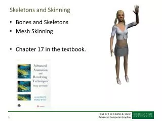
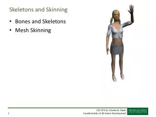
Skeletons • Skeleton: A pose-able framework of joints arranged in a tree structure. The skeleton is used as an invisible armature to manipulate the skin and other geometric data of the character • Joint: A joint allows relative movement within the skeleton. Joints are essentially 4x4 matrix transformations. Joints can be rotational, translational, or some non-realistic types as well • Bone: Bone is really just a synonym for joint for the most part. For example, one might refer to the shoulder joint or upper arm bone (humerus) and mean the same thing
DOFs • Degree of Freedom (DOF): A variable φ describing a particular axis or dimension of movement within a joint • Joints typically have around 1-6 DOFs (φ1…φN) • Changing the DOF values over time results in the animation of the skeleton • In later weeks, we will extend the concept of a DOF to be any animatable parameter within the character rig • Note: in a mathematical sense, a free rigid body has 6 DOFs: 3 for position and 3 for rotation
Joints • Core Joint Data • DOFs (N floats) • Local matrix: L • World matrix: W • Additional Data • Joint offset vector: r • DOF limits (min & max value per DOF) • Type-specific data (rotation/translation axes, constants…) • Tree data (pointers to children, siblings, parent…)
Skeleton Posing Process • Specify all DOF values for the skeleton (done by higher level animation system) • Recursively traverse through the hierarchy starting at the root and use forward kinematics to compute the world matrices (done by skeleton system) • Use world matrices to deform skin & render (done by skin system) Note: the matrices can also be used for other things such as collision detection, FX, etc.
Forward Kinematics • In the recursive tree traversal, each joint first computes its local matrix L based on the values of its DOFs and some formula representative of the joint type: Local matrix L = Ljoint(φ1,φ2,…,φN) • Then, world matrix W is computed by concatenating L with the world matrix of the parent joint World matrix W = L · Wparent
Joint Offsets • It is convenient to have a 3D offset vector r for every joint which represents its pivot point relative to its parent’s matrix
DOF Limits • It is nice to be able to limit a DOF to some range (for example, the elbow could be limited from 0º to 150º) • Usually, in a realistic character, all DOFs will be limited except the ones controlling the root
Skeleton Rigging • Setting up the skeleton is an important and early part of the rigging process • Sometimes, character skeletons are built before the skin, while other times, it is the opposite • To set up a skeleton, an artist uses an interactive tool to: • Construct the tree • Place joint offsets • Configure joint types • Specify joint limits • Possibly more…
Poses • Once the skeleton is set up, one can then adjust each of the DOFs to specify the pose of the skeleton • We can define a pose Φ more formally as a vector of N numbers that maps to a set of DOFs in the skeleton Φ = [φ1 φ2 … φN] • A pose is a convenient unit that can be manipulated by a higher level animation system and then handed down to the skeleton • Usually, each joint will have around 1-6 DOFs, but an entire character might have 100+ DOFs in the skeleton • Keep in mind that DOFs can be also used for things other than joints, as we will learn later…
Rotational Hinge: 1-DOF Universal: 2-DOF Ball & Socket: 3-DOF Euler Angles Quaternions Translational Prismatic: 1-DOF Translational: 3-DOF (or any number) Compound Free Screw Constraint Etc. Non-Rigid Scale Shear Etc. Design your own... Joint Types
Hinge Joints (1-DOF Rotational) • Rotation around the x-axis:
Hinge Joints (1-DOF Rotational) • Rotation around the y-axis:
Hinge Joints (1-DOF Rotational) • Rotation around the z-axis:
Hinge Joints (1-DOF Rotational) • Rotation around an arbitrary axis a:
Universal Joints (2-DOF) • For a 2-DOF joint that first rotates around x and then around y: • Different matrices can be formed for different axis combinations
Ball & Socket (3-DOF) • For a 3-DOF joint that first rotates around x, y, then z: • Different matrices can be formed for different axis combinations
Prismatic Joints (1-DOF Translation) • 1-DOF translation along an arbitrary axis a:
Translational Joints (3-DOF) • For a more general 3-DOF translation:
Other Joints • Compound • Free • Screw • Constraint • Etc. • Non-Rigid • Scale (1 axis, 3 axis, volume preserving…) • Shear • Etc.
Skin CSE169: Computer Animation Instructor: Steve Rotenberg UCSD, Winter 2005
Texture • We may wish to ‘map’ various properties across the polygonal surface • We can do this through texture mapping, or other more general mapping techniques • Usually, this will require explicitly storing texture coordinate information at the vertices • For higher quality rendering, we may combine several different maps in complex ways, each with their own mapping coordinates • Related features include bump mapping, displacement mapping, illumination mapping…
Weighted Blending & Averaging • Weighted sum: • Weighted average: • Convex average:
Rigid Parts • Robots and mechanical creatures can usually be rendered with rigid parts and don’t require a smooth skin • To render rigid parts, each part is transformed by its joint matrix independently • In this situation, every vertex of the character’s geometry is transformed by exactly one matrix where v is defined in joint’s local space
Simple Skin • A simple improvement for low-medium quality characters is to rigidly bind a skin to the skeleton. This means that every vertex of the continuous skin mesh is attached to a joint. • In this method, as with rigid parts, every vertex is transformed exactly once and should therefore have similar performance to rendering with rigid parts.
Smooth Skin • With the smooth skin algorithm, a vertex can be attached to more than one joint with adjustable weights that control how much each joint affects it • Verts rarely need to be attached to more than three joints • Each vertex is transformed a few times and the results are blended • The smooth skin algorithm has many other names: blended skin, skeletal subspace deformation (SSD), multi-matrix skin, matrix palette skinning…
Smooth Skin Algorithm • The deformed vertex position is a weighted average:
Binding Matrices • With rigid parts or simple skin, v can be defined local to the joint that transforms it • With smooth skin, several joints transform a vertex, but it can’t be defined local to all of them • Instead, we must first transform it to be local to the joint that will then transform it to the world • To do this, we use a binding matrix B for each joint that defines where the joint was when the skin was attached and premultiply its inverse with the world matrix:
Normals • To compute shading, we need to transform the normals to world space also • Because the normal is a direction vector, we don’t want it to get the translation from the matrix, so we only need to multiply the normal by the upper 3x3 portion of the matrix • For a normal bound to only one joint:
Normals • For smooth skin, we must blend the normal as with the positions, but the normal must then be renormalized: • If the matrices have non-rigid transformations, then technically, we should use:
Algorithm Overview Skin::Update() (view independent processing) • Compute skinning matrix for each joint: M=B-1·W (you can precompute and store B-1 instead of B) • Loop through vertices and compute blended position & normal Skin::Draw() (view dependent processing) • Set matrix state to Identity (world) • Loop through triangles and draw using world space positions & normals Questions: • Why not deal with B in Skeleton::Update() ? • Why not just transform vertices within Skin::Draw() ?
Rig Data Flow • Input DOFs • Rigging system (skeleton, skin…) • Output renderable mesh (vertices, normals…) Rig
Skeleton Forward Kinematics • Every joint computes a local matrix based on its DOFs and any other constants necessary (joint offsets…) • To find the joint’s world matrix, we compute the dot product of the local matrix with the parent’s world matrix • Normally, we would do this in a depth-first order starting from the root, so that we can be sure that the parent’s world matrix is available when its needed
Smooth Skin Algorithm • The deformed vertex position is a weighted average over all of the joints that the vertex is attached to: • W is a joint’s world matrix and B is a joint’s binding matrix that describes where it’s world matrix was when it was attached to the skin model (at skin creation time) • Each joint transforms the vertex as if it were rigidly attached, and then those results are blended based on user specified weights • All of the weights must add up to 1: • Blending normals is essentially the same, except we transform them as direction vectors (x,y,z,0) and then renormalize the results
Skinning Equations • Skeleton • Skinning
Limitations of Smooth Skin • Smooth skin is very simple and quite fast, but its quality is limited • The main problems are: • Joints tend to collapse as they bend more • Very difficult to get specific control • Unintuitive and difficult to edit • Still, it is built in to most 3D animation packages and has support in both OpenGL and Direct3D • If nothing else, it is a good baseline upon which more complex schemes can be built
Bone Links • To help with the collapsing joint problem, one option is to use bone links • Bone links are extra joints inserted in the skeleton to assist with the skinning • They can be automatically added based on the joint’s range of motion. For example, they could be added so as to prevent any joint from rotating more than 60 degrees. • This is a simple approach used in some real time games, but doesn’t go very far in fixing the other problems with smooth skin.
Shape Interpolation • Another extension to the smooth skinning algorithm is to allow the verts to be modeled at key values along the joints motion • For an elbow, for example, one could model it straight, then model it fully bent • These shapes are interpolated local to the bones before the skinning is applied • We will talk more about this technique in the next lecture
Muscles & Other Effects • One can add custom effects such as muscle bulges as additional joints • For example, the bicep could be a translational or scaling joint that smoothly controls some of the verts in the upper arm. Its motion could be linked to the motion of the elbow rotation. • With this approach, one can also use skin for muscles, fat bulges, facial expressions, and even simple clothing • We will learn more about advanced skinning techniques in a later lecture
Rigging Process • To rig a skinned character, one must have a geometric skin mesh and a skeleton • Usually, the skin is built in a relatively neutral pose, often in a comfortable standing pose • The skeleton, however, might be built in more of a zeropose where the joints DOFs are assumed to be 0, causing a very stiff, straight pose • To attach the skin to the skeleton, the skeleton must first be posed into a binding pose • Once this is done, the verts can be assigned to joints with appropriate weights
Skin Binding • Attaching a skin to a skeleton is not a trivial problem and usually requires automated tools combined with extensive interactive tuning • Binding algorithms typically involve heuristic approaches • Some general approaches: • Containment • Point-to-line mapping • Delaunay tetrahedralization
Containment Binding • With containment binding algorithms, the user manually approximates the body with volume primitives for each bone (cylinders, ellipsoids, spheres…) • The algorithm then tests each vertex against the volumes and attaches it to the best fitting bone • Some containment algorithms attach to only one bone and then use smoothing as a second pass. Others attach to multiple bones directly and set skin weights • For a more automated version, the volumes could be initially set based on the bone lengths and child locations
Point-to-Line Mapping • A simple way to attach a skin is treat each bone as one or more line segments and attach each vertex to the nearest line segment • A bone is made from line segments connecting the joint pivot to the pivots of each child