Download
1 / 34
380 likes | 602 Vues
Lecture 16: Paternity Analysis and Phylogenetics. October 19, 2012. Last Time. Population assignment examples Forensic evidence and individual identity Introduction to paternity analysis. Today. Using F ST to estimate migration Direct estimates of migration: parentage analysis

E N D
Lecture 16: Paternity Analysis and Phylogenetics October 19, 2012
Last Time • Population assignment examples • Forensic evidence and individual identity • Introduction to paternity analysis
Today • Using FST to estimate migration • Direct estimates of migration: parentage analysis • Introduction to phylogenetic analysis
qm m m m m m q0 q0 q0 q0 q0 Island Model of Population Structure Expected Identity by Descent at time t, no migration: IBD due to prior inbreeding IBD due to random mating Incorporating migration: If population size on islands is small, and/or gene flow (m) is low, drift will occur where m is proportion of N that are migrants each generation
Migration-Drift Equilibrium At migration-drift equilibrium: • This aproach is VERY widely used to calculate number of migrants per generation • It is an APPROXIMATION of EQUILIBRIUM conditions under the ISLAND MODEL • Only holds for low Nm • FST=0.01, approximation is Nm = 24.8 • If N=50, actual Nm is 14.6 FST = ft = ft-1 Assuming m2 is small, and ignoring 2m in numerator and denominator:
qm m m m m m q0 q0 q0 q0 q0 Differentiation of Subpopulations • Subpopulations will be more uniform with high levels of gene flow and/or high N • Nm>1 homogenizes populations • Nm<<1 results in fixation of alternate alleles and ultimate differentiation (FST=1) At drift-migration equilibrium:
Limitations of FST • FST is a long, integrated look into the evolutionary/ecological history of a population: may not represent status quo • Assumptions of the model frequently violated: • Island model unrealistic • Selection is often an important factor • Mutation may not be negligible • Sampling error!
Alternatives to FST • Direct measurements of movement: mark-recapture • Genetic structure of paternal and maternal gametes only • Chloroplast and mitochondrial DNA • Pollen gametes • Parentage analysis: direct determination of the parents of particular offspring through DNA fingerprinting
Paternity Exclusion Analysis • Determine multilocus genotypes of all mothers, offspring, and potential fathers • Determine paternal gamete by “subtracting” maternal genotype from that of each offspring. • Infer paternity by comparing the multilocus genotype of all gametes to those of all potential males in the population • Assign paternity if all potential males, except one, can be excluded on the basis of genetic incompatibility with the observed pollen gamete genotype • Unsampled males must be considered
NO NO YES YES YES NO NO YES NO YES YES NO YES YES NO Paternity Exclusion Locus 1 • First step is to determine paternal contribution based on seedling alleles that do not match mother • Notice for locus 3 both alleles match mother, so there are two potential paternal contributions • Male 3 is the putative father because he is the only one that matches paternal contributions at all loci Locus 2 Locus 3
Sweet Simulation of Paternity Analysis • Collected seeds (baby) from a hermaphroditic, self-incompatible plant • Which of the candidate hermaphrodites (you) fathered the seeds? • Six loci with varying numbers of alleles Organize candy into loci (next slide) Determine paternal contribution to offspring by subtracting maternal alleles Exclude potential fathers that don’t have paternal allele Nonexcluded candidate is the father!
Mother and Child Maternal Alleles Paternal Alleles
Alleles versus Loci • For a given number of alleles: one locus with many alleles provides more exclusion power than many loci with few alleles • 10 loci, 2 alleles, Pr = 0.875 • 1 locus, 20 alleles, Pr=0.898 • Uniform allele frequencies provide more power
Characteristics of an ideal genetic marker for paternity analysis • Highly polymorphic, (i.e. with many alleles) • Codominant • Reliable • Low cost • Easy to use for genotyping large numbers of individuals • Mendelian or paternal inheritance
Shortcomings of Paternity Exclusion • Requiring exact matches for potential fathers is excessively stringent • Mutation • Genotyping error • Multiple males may match, but probability of match may differ substantially • No built-in way to deal with cryptic gene flow: case when male matches, but unsampled male may also match • Type I error: wrong father assigned paternity)
Is it possible we’re implicating the wrong father in our paternity exclusion analysis? Look at mismatching loci and the genotypes. Could you have been wrongly excluded?
Probabilistic Approaches • Consider the probability of alternative hypotheses given the data • Probabilities are conditioned based on external evidence (prior probabilities) Probability of hypothesis 1, given the evidence Probability of the evidence, given hypothesis 1 Prior probability of hypothesis 1
Likelihood Approach for Paternity Assignment • Consider two hypotheses: • Alleged father is the true father • A random male from the population is the true father • Calculate a score for each male, reflecting probability he is correct father: where H1 is probability male a is father, H2 is probability male a is not father T is transition probability P is probability of observing the genotype and go,gm and gaare genotypes of offspring, mother, and alleged father
Transition Probabilities Marshall et al. (1998)
LOD Score for Paternity: “Cervus” program • Combine likelihoods across loci by multiplying together • What is a significant LOD? • No good criteria • Use difference between most likely (LOD1), next most likely (LOD2) • Calculate Log Odds Ratio (LOD) Other programs listed at NIST website: http://www.cstl.nist.gov/strbase/kinship.htm#KinshipPrograms
Advantages and Disadvantages of Likelihood • Advantages: • Flexibility: can be extended in many ways • Compensate for errors in genotyping • Incorporate factors influencing mating success: fecundity, distance, and direction • Compensates for lack of exclusion power • Fractional paternity • Disadvantages • Often results in ambiguous paternities • Difficult to determine proper cutoff for LOD score
Summary • Direct assessment of movement is best way to measure gene flow • Parentage analysis is powerful approach to track movements of mates retrospectively • Paternity exclusion is straightforward to apply but may lack power and is confounded by genotyping error • Likelihood-based approaches can be more flexible, but also provide ambiguous answers when power is lacking
Phylogenetics • Study of the evolutionary relationships among individuals, groups, or species • Relationships often represented as dichotomous branching tree • Extremely common approach for detecting and displaying relationships among genotypes • Important in evolution, systematics, and ecology (phylogeography)
O G P C Q H A R S I D J T U K E V L W B X M Y F Z N Ç Evolution Slide adapted from Marta Riutart
O P Q R S T U V W X Y Z Ç What is a phylogeny? • Homology: similarity that is the result of inheritance from a common ancestor Slide adapted from Marta Riutart
Group, cluster, clade Leaves, Operational Taxonomic Units (OTUs) terminal branches node interior branches Phylogenetic Tree Terms A B C D E F G H I J ROOT Slide adapted from Marta Riutart
Bacteria 1 Bacteria 2 Bacteria 3 Eukaryote 1 Eukaryote 2 Eukaryote 3 Eukaryote 4 Bacteria 1 Bacteria 2 Bacteria 3 Eukaryote 1 Eukaryote 2 Eukaryote 3 Eukaryote 4 Tree Topology (Bacteria1,(Bacteria2,Bacteria3),(Eukaryote1,((Eukaryote2,Eukaryote3),Eukaryote4))) Slide adapted from Marta Riutart
Are these trees different? How about these? http://helix.biology.mcmaster.ca
eukaryote eukaryote eukaryote eukaryote Rooted versus Unrooted Trees archaea archaea Unrooted tree archaea Rooted by outgroup bacteria outgroup archaea Monophyletic group archaea archaea eukaryote Monophyletic group eukaryote root eukaryote eukaryote Slide adapted from Marta Riutart
Rooting with D as outgroup A B D A C B C G E F D G F E Slide adapted from Marta Riutart
A B D A C G B E C F G D E A F B C D Now with C as outgroup G F E
Baum et al. Which of these four trees is different?
UPGMA Method • Use all pairwise comparisons to make dendrogram • UPGMA:Unweighted Pairwise Groups Method using Arithmetic Means • Hierarchically link most closely related individuals Also see lab 12