The Concatenated Generalized Matching Law: Influence of Reinforcer Magnitude and Rate on Choice
This summary examines the concatenated Generalized Matching Law (GML) developed by Schneider and Todorov, highlighting the differential effects of reinforcer magnitude and rate on choice behavior. Their findings illustrate that sensitivity to reinforcer rate (0.8-0.9) proves more influential than sensitivity to magnitude (0.5) in shaping choices. The GML encompasses various independent variables (IVs), including delay and arduousness of responses, contributing to a comprehensive understanding of animal behavior and preference. By integrating multiple IVs, this model seeks to predict choice without inherent bias.

The Concatenated Generalized Matching Law: Influence of Reinforcer Magnitude and Rate on Choice
E N D
Presentation Transcript
Schneider (1973) and Todorov (1973) • Version of the GML that describes the effect of reinforcer magnitude on choice • Schneider and Todorov both varied reinforcer magnitude and found that the above equation did describe their data • But sensitivity to magnitude was about 0.5 – much less than sensitivity to rate • Reinforcer rate is more effective at influencing choice than reinforcer magnitude
The concatenated generalized matching law • If we put the GML descriptions of control by rate and magnitude together, we could write the above equation • The sensitivity terms have subscripts identifying the IV they refer to • Each IV controls choice in the same way, but sensitivity to each might differ • Because reinforcer rate affects choice more than reinforcer magnitude does, ar is greater than am
The concatenated generalized matching law • Add a log ratio and a sensitivity term for all the other IVs that affect choice… • Notice that reinforcer delay and response arduousness have reversed log ratios – why? • Sensitivity term: how much influence that IV has on choice • If an IV is constant and equal for both alternatives, its log ratio will be zero and it will drop out of the equation • If an IV is constant and unequal it will produce a bias
The concatenated generalized matching law • e.g., suppose M1 is 6 s access to wheat and M2 is 3 s • We know that am is about 0.5 • The magnitude ratio is 2, so log magnitude ratio is 0.3, so the magnitude term is about 0.5 x 0.3 = 0.15 • So if we vary the reinforcer rates and measure bias, it should be about 0.15 towards the larger magnitude, as long as all the other IVs in the concatenated GML are constant and equal, and there’s no inherent bias
Vollmer and Bouret (2000) College basketball, 3-point shots vs 2-point shots Across players, ratio of shots attempted (responses) slightly undermatched ratio of successful shots (reinforcer rate) Bias in favor of 3-point shots (reinforcer magnitude)
The concatenated generalized matching law • This is an efficient way to write the concatenated GML. The symbol S means “the sum of” • X is any independent variable that affects choice • Predicted log response ratio is the sum of all the log independent-variable ratios multiplied by their sensitivities • There’s no bias term in the equation • When all the IVs that affect choice have been discovered, there will be no inherent bias
The concatenated generalized matching law • Looking at sensitivities to different independent variables • Already seen that sensitivity to : • reinforcer rate is about 0.8 to 0.9 • reinforcer magnitude is about 0.5 • Now, two more IVs – reinforcer delay and response force requirement (manipulating the arduousness of a response)
Response force: Hunter and Davison (1982) • Varied both reinforcer rate in concurrent VI VI and the force required for a key-peck to be counted as a response • Response measures: ar = 0.88, aA = 0.71 • Time measures: ar = 0.98, aA = 0.41 • Force required affected choice less than reinforcer rate • Sensitivities measured using time allocation aren’t always higher than for response allocation • Thorough test of the concatenated GML, fitted the data very well
Rf magnitude: Elliffe, Davison, Landon (2008) • What about with other variables? • Both reinforcer rate and magnitude varied thoroughly • The concatenated GML fitted the data very well, but • Sensitivity to rate was highest when the magnitudes were equal • Sensitivity to magnitude was highest when the rates were equal • Interaction between a values • The CGML can’t be exactly right • probably near enough for predicting behavior in practical terms
Reinforcer delay • The first experiment on this (Chung & Herrnstein, 1967) reported strict matching to relative delay (ad = 1) • But a more thorough later experiment (Williams & Fantino, 1978) found that sensitivity increased with the average delay • This shouldn’t happen according to the GML – sensitivity should stay constant for a particular IV
Assessing preference: reinforcer quality • Testing food preference • Arranging each as a reinforcer for a different response • Varying reinforcer rates • Bias will reflect preference for one or other food, because it will be affected by the log quality ratio • This is the same logic that Hollard and Davison used with food v EBS • Matthews and Temple (1979): cow feeds • Preference for crushed barley
Assessing Reinforcer Quality • Important to use dependent schedules • If you use independent schedules the animal will respond more for the preferred food (say, Q1) • and so its reinforcer rate for that food (R1) will increase • so log (R1/R2) increases • and that increases preference more • so log (R1/R2) increases more • And so on. Can have an apparently very strong preference caused by the animal receiving that food at a higher rate • Pet-food advertisements • Reinforcer preference assessments
Summary • Generalized matching seems to describe choice well in a wide variety of situations – different species, response, reinforcers • It says that different IVs to do with responses and reinforcers all affect choice in the same way … • But that some of them are more effective than others, as measured by their different sensitivity values • It’s the best, most widely applicable, description of choice that we have at the moment • But is it a theory of choice? Why should it happen? • Is Baum’s idea that it’s really ‘failed strict matching’ right? Or is it an outcome of some other mechanism for choice, like maximization?
Experimental Analysis of Choice Methods: concurrent schedules, concurrent chains, delay discounting, foraging contingencies, behavioral economic contingencies. Models and Issues: matching/melioration, maximizing/optimality, hyperbolic discounting, behavioral economic/ecological models, behavior momentum, molar versus molecular issue, concepts of response strength. Applications: self-control, drug abuse, gambling, risk, economics, behavioral ecology, social/political decision making.
Melioration: A Theory of Matching “To make better”: Behavior shifts to the higher return (lower cost) or equal local rates of reinforcement. (R1 / R2) = (r1 / r2), or (r1 / R1) = (r2 / R2) (reinforcers per response, i.e., return). (T1 / T2) = (r1 / r2), or (r1 / T1) = (r2 / T2) (local rate of reinforcement).
Example: Conc VI 30” VI 120” Suppose in the first hour of exposure 1000 responses were emitted to each alternative: (VI 30”) r1 / R1 = (120 rfs / 1000 resps). Return = 0.120 (VI 120”) r2 / R2 = (30 rfs / 1000 resps). Return = 0.03 Ultimately behavior will shift toward the higher return. What will be the result? 120 / (1000 + x) = 30 / (1000 – x); x = 600. 120 / 1600 = 30 / 400 i.e., matching (80% responses on VI 30” alternative). Return = 0.075 rfs/resp on each alternative.
What about VR30 VR120? • How does matching say behavior will be allocated?
Problem: Conc VR 30 VR 120 ALL responses will ultimately be made to the VR 30 alternative. This is consistent with matching, but same would be said if all the responses were made to the VR 120 alternative. But melioration can predict which alternative should receive all the responses: VR 30: r1/ R1 = 1/30; VR 120: r2/ R2 = 1/120. These cannot change, so shifting to the higher return means all the responses will go to VR 30 alternative.
And VR 20 – VI 60? • What would an optimal pattern of response be?
Overall • Mixed bag of results • Some optimization • Some melioration • Something else at play? • Molar theories • Matching, melioration, optimization • Molecular theory • Momentary maximization theory
A Thought Experiment • 2 doors • .1 and .2 probability of getting a dollar respectively • Can get a dollar behind both doors on the same trial • Dollars stay there until collected, but never more than 1 dollar per door. • What order of doors do you choose?
Patterns in the Data • If choices are made moment by moment, should be orderly patterns in the choices: 2, 2, 1, 2, 2, 1… • Results mixed but promising results when using time as the measure
What Works Best Right Now • Maximizing local rates and moment to moment choices can lower overall reinforcement rate. • Short-term vs. long-term
Next Time: • Delay and self-control
A critical fact about self control: Preference reversal In positive self control, the further you are away from the smaller and larger reinforcers, the more likely you are to accept the larger, more delayed reinforcers. But, the closer you get to the first one, the more likely you are to chose the smaller, more immediate one. Preference thus reverses as you make your choice further and further away from the reinforcers. 30
Friday night: “Alright, I am setting my alarm clock to wake me up at 6.00 am tomorrow morning, and then I’ll go jogging.” ... Saturday 6.00 am: “Hmm….maybe not today.” 31
Ainslie-Rachlin theory – an analogy Rachlin (1970, 1974), Ainslie (1975) Preference reversal: The analogy is simply looking at tall buildings as you are walking towards them. From far away, you can see the tall building in the distance. But as you get closer, you can't see it any more, just the shorter building closer to you. So, if you are looking for the tallest building, the highest hill, the largest reinforcer, then you chose the bigger one if you are far away. But if you are close, you choose the smaller one. 32
Assume: At the moment in time when we make the choice, we choose the reinforcer that has the highest current value... To be able to understand why preference reversal occurs, we need to know how the value of a reinforcer changes the time by which it is delayed... Outside the laboratory, the majority of reinforcers are delayed. Studying the effects of delayed reinforcers is therefore very important. 34
Basically, the effects that reinforcers have on behaviour decrease -- rapidly -- when the reinforcers are more and more delayed after the reinforced response. This is how reinforcer value generally changes with delay: 35
Studying preference of delayed reinforcers Humans: - verbal reports at different points in time - “what if” questions Humans AND nonhumans: A. Concurrent chains B: Titration All are choice techniques. 36
A. Concurrent chains Concurrent chains are simply concurrent schedules -- usually concurrent equal VI VI -- in which reinforcers are delayed. When a response is reinforced, usually both concurrent schedules stop and become unavailable, and a delay starts. Sometimes the delays are in blackout with no response required to get the final reinforcer (an FT schedule); Sometimes the delays are actually schedules, with an associated stimulus, like an FI schedule, that requires responding. 37
Initial links, Choice phase W W Conc VI VI W W W W Terminal links, Outcome phase VI a s VI b s Food Food The concurrent-chain procedure 38
An example of a concurrent-chain experiment MacEwen (1972) investigated choice between two terminal-link FI and and two terminal-link VI schedules, one of which was always twice as long as the other. The initial links were always concurrent VI 60-s VI 60-s schedules. 39
The terminal-link schedules were: Constant reinforcer (delay and immediacy) ratio in the terminal links – all immediacy ratios are 2:1. 40
From the generalised matching law, we would expect: If ad was constant, then because D2/D1 was kept constant, we would expect no change in choice with changes in the absolute size of the delays. D2/D1 was kept constant throughout. 42
But choice did change, so ad did NOT remain constant: A serious problem for the generalised matching law. 43
B: Titration - Finding the point of preference reversal The titration procedure was introduced by Mazur: - one standard (constant) delay and - one adjusting delay. These may differ in what schedule they are (e.g., FT versus VT with the same size reinforcers for both), or they may be the same schedule (both FT, say) with different magnitudes of reinforcers. What the procedure does is to find the value of the adjusting delay that is equally preferred to the standard delay -- the indifference point in choice. 44
For example: - reinforcer magnitudes are the same - standard schedule is VT 30 s - adjusting schedule is FT How long would the FT schedule need to become to make preference equal? Answer: Probably about FT 20 s. Concurrent chains give the same result. Animals prefer the risky option (hyperbolic averaging). 45
Titration: Procedure Trials are in blocks of 4. The first 2 are forced choice, randomly one to each alternative The last 2 are free choice. If, on the last 2 trials, it chooses the adjusting schedule twice, the adjusting schedule is increased by a small amount. If it chooses the standard twice, the adjusting schedule is decreased by a small amount. If equal choice (1 of each) -- no change (von Bekesy procedure in audition) 46
Mazur's titration procedure Why the post-reinforcer blackout? ITI W W W Trial start W W W Peck Choice W W W Standard delay + red houselight Adjusting delay + green houselight 2-s food, BO 6-s food 47
Animal research: Preference reversal Green, Fisher, Perlow, & Sherman (1981) Choice between a 2-s and a 6-s reinforcer. Larger reinforcer delayed 4 s more than the smaller. Choice response (across conditions) required from 2 to 28 s before the smaller reinforcer. We will call this time T. 48
Large rf Small rf choice 4 s 28 s T 2 s 49
Large rf Small rf choice 4 s 28 s T 2 s 50