Lecture 8 Cost Curves

1. Lecture 8Cost Curves

2. Total Cost and its Break Down Total Cost = Total Fixed + Total Variable Cost Cost Fixed cost is any cost that does not depend on the firm’s level of output. These costs are incurred even if the firm is producing nothing. Variable cost is a cost that depends on the level of production chosen. Total cost is the sum total fixed cost and total variable cost.

3. Average Cost and its Break Down Average Cost, is total cost divided by quantity of output produced. AC = TC/Q Average fixed cost is the fixed cost per unit of output. AFC = FC/Q Average variable cost is the variable cost per unit of output. AVC = VC/Q AC= AVC+ AFC

4. Derivation of Marginal Cost fromTotal Cost Marginal cost measures the additional cost of inputs required to produce each successive unit of output. MC = (Change in total cost)/(Change in quantity) = ΔTC/ΔQ.

5. Example of Different Costs

6. Total, Average, and Marginal Revenue for a Competitive Firm

7. Profit-maximization condition is: MR = MC

8. Economies of Scale Economies of scale, in microeconomics, refers to the cost advantages that a business obtains due to expansion of business. The decrease in unit cost of a product or service resulting from large-scale operations is known economies of scale. 1) Economies of scale : When long-run average total cost declines as output increases, there are said to be economies of scale. 2) Diseconomies of scale: When long-run average total cost rises as output increases, there are said to be diseconomies of scale. 3) Constant returns to scale: When long-run average total cost does not vary with the level of output, there are said to be constant returns to scale.

9. Example: Suppose Ford is considering its costs for different output level. Ford will have economies of scale at low levels of output, constant returns to scale at intermediate levels of output, and diseconomies of scale at high levels of output. What might cause economies or diseconomies of scale? Economies of scale often arise because higher production levels allow specialization among workers, which permits each worker to become better at his or her assigned tasks. For instance, modern assembly-line production requires a large number of workers. If Ford were producing only a small quantity of cars, it could not take advantage of this approach and would have higher average total cost. Diseconomies of scale can arise because of coordination problems that are inherent in any large organization. The more cars Ford produces, the more stretched the management team becomes, and the less effective the managers become at keeping costs down. This analysis shows why long-run average-total-cost curves are often U shaped. At low levels of production, the firm benefits from increased size because it can take advantage of greater specialization. Coordination problems, meanwhile, are not yet acute. By contrast, at high levels of production, the benefits of specialization have already been realized, and coordination problems become more severe as the firm grows larger. Thus, long-run average total cost is falling at low levels of production because of increasing specialization and rising at high levels of production because of increasing coordination problems.

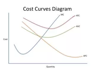
10. Average Cost Curve is U shaped • At the initial level of output, the firm has economies of scale that means cost falls as the quantity of output increases (firm is operating in a downward sloping region of the average cost curve). • Then after a certain output level the firm has a constant return to scale that means average cost stays the same as the quantity of output changes ( firm will operate at the minimum point of AC curve). • Then at the higher output level from the minimum point the firm will have diseconomies of scale that means average cost rises as the quantity of output increases ( firm will operate in the upward sloping part of average cost curve). • So the average cost curve is U shaped. • The bottom of the U-shape occurs at the quantity that minimizes average total cost. This quantity is sometimes called the efficient scale of the firm.

11. Relation between AC and MC Curve Relationship: MC curve goes through the minimum point of AC curve. • At output less than the minimum point of AC curve, marginal cost isless thanaverage total cost and average total cost is falling. • And at output greater than the minimum point of AC curve, marginal cost isgreater thanaverage total cost and average total cost is rising. • At the minimum point of AC curve, average total cost is equal tomarginal cost. • Example: To see why this happens, consider an analogy. Average total cost is like your cumulative grade point average. Marginal cost is like the grade in the next course you will take. If your grade in your next course is less than your grade point average, your grade point average will fall. If your grade in your next course is higher than your grade point average, your grade point average will rise.

12. The Relationship Between the Average Total Cost and the Marginal Cost Curves