Thermodynamics of Multi-component Systems
270 likes | 698 Vues
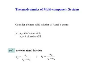
Thermodynamics of Multi-component Systems. Consider a binary solid solution of A and B atoms:. Let n A = # of moles of A n B = # of moles of B. def:. mole(or atom) fraction. ;. G B. G 1. G A. 0. 1. X B. Consider n A moles of A and n B moles of B. Before they are mixed:.

Thermodynamics of Multi-component Systems
E N D
Presentation Transcript
Thermodynamics of Multi-component Systems Consider a binary solid solution of A and B atoms: Let nA= # of moles of A nB= # of moles of B def: mole(or atom) fraction ;
GB G1 GA 0 1 XB Consider nAmoles of A and nBmoles of B. Before they are mixed: Variation of the free energy before mixing with alloy composition. XB moles of B XA moles of A
The Free Energy of the system changes on mixing MIX fixed T XB moles of B XA moles of A 1 mole of solid solution
Since Defining Lets consider each of the terms recall that for condensed systems ΔH≈ ΔU and so Δ Hmix= heat of solution ≈ change in internal energy before and after mixing. Hmix-
Smix- change in entropy due to mixing. Take the mixing to be “perfect”i.e., random solid solution Smix= (molar) Configurational entropy Boltzmann’s Eqn. W= # of distinguishable ways of arranging the atoms → “randomness” The number of A atoms and B atoms in the mixture is: NA = nANa NB = nBNa Na , Avogadro’s number From combinatorial mathematics:
ln W can be approximated usingStirling’s approximation, , and using, Nak = R, where R is the gas constant, we obtain, Let’s Re-examine the Hmixterm: 2 models • Ideal solution model • Regular solution model Ideal Solutions Hmix= 0 Physically this means the A atoms interact with the B atoms as if they are A and vice versa.
The only contribution to alterations in the Gibbs potential is in the configurational entropy i.e., Examples: • Solution of two isotopes of the same element • Low pressure gas mixtures • Many dilute ( xA<< xB or xB<< xA)condensed phase solutions.
Recall that the total free energy of the solution G GB G1 Gmix 0 1 XB Low T GA -TSmix High T Gmix 0 1 XB
Regular Solutions Assume a random solid solution and consider how the A&B atoms interact. MIX fixed T XB moles of B XA moles of A 1 mole of solid solution
The Regular Solution model assumes only nearest-neighbor interactions, pairwise. “Quasichemical” model Bond energy Bond energy Bond energy In a general the interaction of an A atom with another A atom or a B atom depends upon • interatomic distance • atomic identity • 2nd, 3rd, … next –near-neighbor identity and distances. Assume the interatomic distance set by the lattice sites. Let : Note that all the V’sare < 0.
Consider a lattice of N sites with Z nearest-neighbors per site. : Each of the N atoms has Z bonds so that there are bonds in the lattice. Division by 2 is for double counting. Let PAA be the probability that any bond in the lattice is an A-A bond: then and so
The energy for the mixed solution is prior to mixing and
combining terms & using xA + xB = 1 where Notice the ΔHmix can be either positive or negative. ΔHmix > 0, > 0 and VAB > 1/2 (VAA+ VBB) from ΔGmix = ΔHmix – TΔSmix At low temps clustering of Asand Bsresult, i.e., “phase separation”.
for ΔHmix < 0, < 0 and VAB < 1/2 (VAA+ VBB) The A atoms are happier with B atoms as nearest-neighbors. Short range ordering i.e., PAB is increases over the random value. For a Regular Solution
xB → 0 1 –TΔSmix ΔGmix ΔHm ΔGm Note 2 minima change in curvature 2 pts of inflection. ΔHmix ΔGmix 0 1 xB → ΔGmix –TΔSmix Variation of ΔGmix with composition < 0 > 0 T < TC
XB → 0 1 ΔGmix T < Tc T = Tc As T increases, the –TΔS term begins to dominate. The inflection pt. & extremum merge the critical temperature: