Download
1 / 33
330 likes | 556 Vues
Cylindrical Reflector SKA Update. John Bunton CSIRO Telecommunications and Industrial Physics. Overview. Concept Linefeed Costs Fields of view Applications. Making the desert bloom -. With Cylindrical Reflectors. SKA compact core?.

E N D
Cylindrical Reflector SKA Update John Bunton CSIRO Telecommunications and Industrial Physics
Overview • Concept • Linefeed • Costs • Fields of view • Applications
SKA compact core? Solar energy collection using cylindrical reflectors. Collecting area over 1 km2 Confirms original reflector estimates for cylindrical concept: ~$235m2 at 6 GHz Includes foundations Comparable 12 m (preloaded) ~$530m2
Philosophy • Paraboloids best at high frequencies, Maximises the area of each detector/feed • At least 4400 feeds in the SKA • Cylindrical Reflector • Single axis reflector cheaper than two axis • large FOV compared to paraboloids • Reduced feed count compared to phased arrays • Phased arrays good at low frequencies, feeds are cheap and large effective area, large FOV • No. of feeds increases quadratically with frequency
History • Cylindrical Reflector (64m dish = 3,200 m2) • 1958 - 178MHz, Radio Star Interfer. 10,000 m2, • 1967 ~400MHz • Northern Cross 31,000 m2 • Ooty 16,000 m2 • Molonglo 40,000 m2 • 1980 - 843 MHz, MOST 19,000 m2 • Extrapolating to 2010 we could have a university instrument with 20,000 m2 at 6 GHz • Electronics cost and LNA noise the problem
Today • LNA problem is being solved • Simple SiGe LNA uncooled, 47K at 2 GHz • All concepts have multiple receiver • No longer just a problem for cylinders • Electronics cost keeps on coming down • E.g. 4560 baseline correlator ~$4k • Moore’s Law should continue to 2010 • Full digital beamforming possible • Solves the problem of meridian distance steering • Cylindrical reflectors again become a viable solution
Cylindrical Reflector Concept • Original white paper 2002, Update presented here • Offset fed cylindrical reflector • Low cost collecting area • 111 by 15 metres (1650 m2) • Multiple Line feeds in the focal plane • Each 3:1 in frequency • Low spillover for central part of linefeed • Linefeed 100m • reduced spillover • Aperture efficiency ~69% • Spillover 3-4K
Array Concept • 1 km compact core filling factor ~0.3, UV filling ~100% • 3 km doubly replicate compact core, min UV filling ~50% • 10 km array asymmetric to save cabling. 1 km compact core replicated within any 2x2 km area of UV space. 4% UV filling of remaining 75%. • 31 km array –UV filling instantaneously greater than .4% in any 1km2
Odds and Ends • Sub 10s response time with three sub-arrays • Antenna - 4 section each independently steerable • End sections, one observes before transit and the other after. Middle sections close to transit. • Accessible sky ~200 deg2 at 1.4 GHz - 4 independent meridian angles (declinations) • Also sub-arrays of antenna stations • Tied arrays probably only central core • 100 to 400 pencil beams (bandwidth 4.9GHz) • Sampling time after first filterbanks - 0.6 to 5μs
Linefeed • Focal area of offset fed cylinder is large – multiple linefeeds (James and Parfitt) • Use Aperture tile array technology for focal plane array (5 elements wide by n long) • Allows reasonable field match • Resulting in good efficiency and polarisation • Mitigate residual polarisation errors by aligning feeds at 45o to the axis of the cylinder • Plus calibration
Multiple Linefeeds • Need multiple line feeds to cover full frequency range (each at ~3:1) • Will have three or more line feeds in the focal plane at any one time. However fields of view may not overlap. (more linefeed work needed here) • Can divide beamforming and signal transmission resources between the individual IFs from all linefeeds.
Linefeed cost reduction • Increased bandwidth from 2:1 to 3:1 • Reduces number of linefeeds - save 25% • Linefeed cost broken down into hardware and electronics. • Hardware cost increases slowly with frequency • Reduced cost at high frequencies • As foreshadowed in white paper use ASICs instead of FPGA • Five times cost reduction of electronics
Antenna station costs • Competitive to 20 GHz+ • Station electronics and fibre, (linefeed & beamformer) half the cost • Cheapest solution below 10 GHz • See poster for other concepts
Cylindrical Cost Breakdown • 22 GHz cylindrical $760M for antenna stations • Total cost ~$1.3 billion
Hybrid SKA • 500 MHz cylindrical reflector $150m 1km2 • + 3 GHz cylindrical reflector $290M 1km2 • + 34 GHz hydroformed $400M 0.25km2 • Antenna station cost $840M • Total cost similar to 22 GHz cylinder • Area 2 km2below 500 MHz • A/Tsys = 10,000 m2/K 0.25 GHz • A/Tsys = 30,000 m2/K 0.5 to 3 GHz • A/Tsys = 10,000 m2/K above 3 GHz.
Element Field of View • This the FOV of a single feed element. • In one directions same as phased arrays • ~120 degrees (electronic beamwidth) • but sensitivity proportional to cos(MD) • FOV increases with MD (MD ~ HA) • Constrained by the reflector in orthogonal direction (reflector beamwidth) • 1.4/ν degrees (ν in GHz) for 15m reflector
Element FOV on the sky FOV covers large range of MD (~HA) Adjacent beams approximately sidereal at transit Beams rotate at large HAs giving access to large areas of sky Example – Hatched area available during 10 hour observation of a source at DEC-30o
Antenna Field of View • Field of view defined by RF beamformer • As frequency increases must limit front end electronics. • RF beamforming • For SKA • 120o below 1.5GHz = elemental FOV • 170o/ νfor frequencies from 1.5 to 7GHz • 51o/ νfor frequencies above 7GHz • E.g. at 10GHZ the antenna FOV is 5o x .14o • 30 times larger than a 12m paraboloid
Imaging Field of View • Field of view defined by signal from antenna station • Have fixed total bandwidth from antenna. • For SKA 64 full bandwidth signals (core antennas) • Allows 8 circular beams or 64 fanbeams • With 64 full bandwidth fanbeams • All beams can be imaged • Their total area is the imaging FOV
Field of View in MD Elemental FOV Antenna FOV Equals elemental FOV below 1.5GHz Imaging FOV Multiple beams within Antenna FOV after digital beamforming
FOV – Bandwidth trade-off • Full bandwidth of 4.9 GHz not always needed • Particularly at lower frequencies • 1.5 GHz nominal bandwidth is 0.8GHz • Can fit of six (6) 0.8GHz signals in place of a single full bandwidth signal • Increases number of beams and FOV by 6 • Imaging FOV = 48 deg2 at 1.4GHz • Doubling the bandwidth to 1.6 GHz gives • Imaging FOV = 1.9 deg2 at 5GHz • Product of FOV and bandwidth constant
48 Square Degrees??? • Correlator efficiency proportional to size of filled aperture • Cylindrical reflector aperture 15 times greater than 12m Paraboloid • Bandwidth trade-off gives a factor of 6 • Not possible unless Antenna FOV>Imaging FOV • But cylindrical has Tsys twice as great as 12 m paraboloid with cooled LNA • Increases correlator size by factor of 4 • Cylindrical Correlator gives a 15*6/4 = 22.5 greater imaging area at 1.4 GHz per $/watt/MIP
SKAMP – SKA Molonglo Demonstrator • see posters for details on correlator and update • Continuum correlator • New 4560 baselines using 18m sections • Old system 64 fanbeams, two 800 m sections • More correlation because of smaller sections • And will give greater dynamic range • Spectral Line correlator • Wideband line feed • Work has started
Field of View – reduced BW Antenna FOV Imaging FOV 0.8GHz Imaging FOV 1.6GHz Imaging FOV Full bandwidth Original Specs
Daily All Sky Monitoring • At 1.4 GHz and a bandwidth of 400MHz • Image 96 deg2 with one minute integration • Time to image 30,000 deg2 is 5.3 hours • Observe in ~1.5 hour sessions 4 times a day • Resolution 1 arcsec with 105 dynamic range • Sensitivity 6μJy (5σ) • Compute power to generate images • Wait for Moore’s law or • Build FPGA/ASIC compute engine
Daily All Sky Monitoring • Daily monitoring and detection of • AGN variability • Star Burst galaxies Supernova • GRB • IDV • ESE …. • See poster Minh Huynh (ANU) et al.], noise 11μJy
Simultaneous Best Effort • Many programs do not use all resources • E.g. target observing of compact sources • Antenna FOV is large • 120 deg2 @1.4 GHz, 0.7 deg2 @ 10 GHz • List all non-time critical observations • If observations is with antenna FOV and bandwidth resources available then proceed • System will make “Best Effort” get your observing program done. Target leftover fields • Can maximise use of SKA resources • Correlator, transmission bandwidth
Simultaneous HI survey • For z=3 antenna FOV is large - 500 deg2 • Choose 100 uniformly distributed field centres • At least one is in the antenna FOV all the time • Independent of targeted observing • Allocate 8 beams for circular FOV - 8 deg2 • After five years av. 400 hours on each field • 10μJy (5σ) at 20 km/s velocity resolution • Redshift for 100s million galaxies • Directlytrace the large scale structure of the Universe.
SKA speed • Fast surveys and simultaneous “best effort” observing • Instrument has very high observing throughput • Surveys an order of magnitude faster. • Other observing modes 2 to 5 times faster • If average speed is 4 times faster • Equivalent to two times increase in sensitivity for non-transient sources. • A/Tsys ≡ 40,000 m2/K
Conclusion A cylindrical reflector offers the unique combination of • High frequency operation to 22 GHz+ • Large imaging FOV • Fastest survey speeds • Daily all sky 1.4 GHz surveys • Large antenna FOV • Multiple simultaneous observation • Example piggy back deep z=3 HI survey • High speed equivalent to higher sensitivity