Download
1 / 24
250 likes | 317 Vues
Learn about estimating error variances in Ordinary Least Squares (OLS) regression using Gauss-Markov Assumption and homoskedasticity. Understand how sample variances affect estimator efficiency and standard errors calculation.

E N D
2.5 Variances of the OLS Estimators -We have proven that the sampling distribution of OLS estimates (B0hat and B1hat) are centered around the true value -How FAR are they distributed around the true values? -The best estimator will be most narrowly distributed around the true values -To determine the best estimator, we must calculate OLS variance or standard deviation -recall that standard deviation is the square root of the variance.
Gauss-Markov Assumption SLR.5(Homoskedasticity) The error u has the same variance given any value of the explanatory variable. In other words,
Gauss-Markov Assumption SLR.5(Homoskedasticity) -While variance can be calculated via assumptions SLR.1 to SLR.4, this is very complicated -The traditional simplifying assumption is homoskedasticity, or that the unobservable error, u, has a CONSTANT VARIANCE -Note that SLR.5 has no impact on unbiasness -SLR.5 simply simplifies variance calculations and gives OLS certain efficiency properties
Gauss-Markov Assumption SLR.5(Homoskedasticity) -While assuming x and u are independent will also simplify matters, independence is too strong an assumption -Note that:
Gauss-Markov Assumption SLR.5(Homoskedasticity) -if the variance is constant given x, it is always constant -Therefore: -σ2 is also called the ERROR VARIANCE or DISTURBANCE VARIANCE
Gauss-Markov Assumption SLR.5(Homoskedasticity) -SLR.4 and SLR.5 can be rewritten as conditions of y (using the fact we expect the error to be zero and y only varies due to the error)
Heteroskedastistic Example -here it is assumed that weight is a function of income -SLR.5 requires that: • Consider the following model: -but income affects weight range -rich people can both afford fatty foods and expensive weight loss -HETEROSKEDATICITY is present
Theorem 2.2(Sampling Variances of the OLS Estimators) Using assumptions SLR.1 through SLR.5, Where these are conditional on sample values {x1,….,xn}
Theorem 2.2 Proof From OLS’s unbiasedness we know, -we know that B1 is a constant and SST and d are non-random, therefore:
Theorem 2.2 Notes -(2.57) and (2.58) are “standard” ols variances which are NOT valid if heteroskedasticity is present 1) Larger error variances increase B1’s variance -more variance in y’s determinants make B1 harder to estimate 2) Larger x variances decrease B1’s variance -more variance in x makes OLS easier to accurately plot 3) Bigger sample size increases x’s variation -therefore bigger sample size decreases B1’s variation
Theorem 2.2 Notes -to get the best estimate of B1, we should choose x to be as spread out as possible -this is most easily done by obtaining a large sample size -large sample sizes aren’t always possible -In order to conduct tests and create confidence intervals, we need the STANDARD DEVIATIONS of B1hat and B2hat -these are simply the square roots of the variances
2.5 Estimating the Error Variance Unfortunately, we rarely know σ2, although we can use data to estimate it -recall that the error term comes from the population equation: -recall that residuals come from the estimated equation: -errors aren’t observable and residuals are calculated from data
2.5 Estimating the Error Variance These two formulas combine to give us: -Furthermore, an unbiased estimator of σ2 is: -But we don’t have data on ui, we only have data on uihat
2.5 Estimating the Error Variance A true estimator of σ2 using uihat is: -Unfortunately this estimator is biased as it doesn’t account for two OLS restrictions:
2.5 Estimating the Error Variance -Since we have two different OLS restrictions, if we have n-2 of the residuals, we can then calculate the remaining 2 residuals that satisfy the restrictions -While the errors have n degrees of freedom, residuals have n-2 degrees of freedom -an unbiased estimator of σ2 takes this into account:
Theorem 2.3(Unbiased Estimation of σ2) Using assumptions SLR.1 through SLR.5,
Theorem 2.3 Proof If we average (2.59) and remember that OLS residuals average to zero we get: Subtracting this from (2.59) we get:
Theorem 2.3 Proof Squaring, we get: Summing, we get:
Theorem 2.3 Proof Expectations and statistics give us: Given (2.61), we now prove the theorem since
2.5 Standard Error -Given (2.57) and (2.58) we now have unbiased estimators of the variance of B1hat and B0hat -furthermore, we can estimate σ as -which is called the STANDARD ERROR OF THE REGRESSION (SER) or the STANDARD ERROR OF THE ESTIMATE (Shazam) -although σhat is not an unbiased estimator, it is consistent and appropriate to our needs
2.5 Standard Error -since σhat estimates u’s standard deviation, it in turn estimates y’s standard deviation when x is factored out -the natural estimator of sd(B1hat) is: -which is called the STANDARD ERROR of B1hat (se(B1hat)) -note that this is a random variable as σhat varies across samples -replacing σ with σhat creates se(B0hat)
2.6 Regression through the Origin -sometimes it makes sense to impose the restriction that when x=0, we also expect y=0 Examples: -Calorie intake and weight gain -Credit card debt and monthly payments -Amount of House watched and how cool you are -Number of classes attended and number of notes taken
2.6 Regression through the Origin -this restriction sets our typical B0hat equal to zero and creates the following line: -where the tilde’s distinguish this problem from the typical OLS estimation -since this line passes through (0,0), it is called a REGRESSION THROUGH THE ORIGIN -since the line is forced to go through a point, B1tilde is a BIASED estimator of B1
-our estimate of B1tilde comes from minimizing the sum of our new squared residuals: 2.6 Regression through the Origin -through the First Order Condition, we get: -which solves to -note that all x cannot equal zero and if xbar equals zero, B1tide equals B1hat