Predicate Logic with Definitions and the General Concept of Algorithm
280 likes | 506 Vues
Predicate Logic with Definitions and the General Concept of Algorithm. Victor Makarov New York, USA http://mysite.verizon.net/resox8fn/vm.htm. Abstract. Predicate Logic with Definitions (D-Logic or DL) is based on First-Order Logic.

Predicate Logic with Definitions and the General Concept of Algorithm
E N D
Presentation Transcript
Predicate Logic with Definitions and the General Concept of Algorithm Victor Makarov New York, USA http://mysite.verizon.net/resox8fn/vm.htm
Abstract • Predicate Logic with Definitions (D-Logic or DL) is based on First-Order Logic. • Its main syntactic constructions are terms, formulas and definitions. • DL can be used for formal writing mathematical definitions. • An algorithm is a mathematical definition of some special kind. • It means that DL can be also used as an algorithmic language
Outline • Practical Formalization of Mathematics. • Mathematical Theories and Object-Oriented Programming. • Predicate Logic with Definitions is based on the First-Order Logic. • Modification #1: Primitive Definitions. • Modification #2: Substitution as a part of the logical language, not a meta-language. • Mathematical Definitions. • An Algorithm is a Mathematical Definition of a special kind • Abstract State Machines
is expressing mathematics, that is, mathematical definitions, theorems and proofs in a (usually small and simple) precisely defined formal language. “Precisely defined” means that the language actually is a formal logical system. Following to V.M Glushkov, we can call such a language as a practical formal mathematical language. Practical Formalization of Mathematics
Mathematical definitions and proofs are written in mathematical theories. So the first step in the design of a formal mathematical language is to answer the question: What is a Mathematical Theory? What is a Mathematical Theory?
The Answer (J. A. Dieudonne) A mathematical theory T is an extension of the first order theory ZFC (Zermelo-Fraenkel set theory with the Axiom of Choice) by adding to ZFC some new constants c1, … , ck and an axiom A(c1, … , ck ). The following syntax is used in DL (theory definition): T : def[c1, … , ck ; A]
A model M of the mathematical theory T is a tuple (z1, … , zk) such that the formula A(z1, …, zk) is a theorem in ZFC. In DL “M T” means “M is a model T”. If P(c1, … , ck) is a theorem in T and M is a model of T then the formula P(z1, … , zk) is also a theorem. P & (M T) M.P M.P is an abbreviation of Subst(P, T, M) M.P is an “object-oriented” notation (C++, Java) If the theory T has a model, than it is consistent. M T E[T] Models of Mathematical Theories
Mathematics and Object-Oriented Programming Note the similarity between the basic mathematical notions and the basic notions of Object-Oriented Programming (OOP): • Mathematical Theory : Class in OOP • A model of the theory : An Instance of the class • A theorem of the theory : A Class invariant
In June 2000, at the annual meeting of the Association for Symbolic Logic (the panel discussion on “The Prospects for Mathematical Logic in the 21st Century”), Sam Buss made the following prediction: Sam Buss’ Prediction
Prediction #3 Computer databases of mathematical knowledge will contain, organize, and retrieve most of the known mathematical literature, by 2030 10 years.
The first step in fulfilling this prediction is to design a formal language which can faithfully represent mathematical objects and constructions in a flexible, extensible way. Perhaps an object-oriented language would be a good choice for this; however, present-day object-oriented languages are not adequate for representing mathematical objects.” Sam Buss’ Prediction (continued)
Predicate Logic with Definitions (D-Logic or DL) • Predicate Logic with Definitions = • Classical (First-Order) Predicate Logic + • Primitive Definitions + • Symbols for Substitution + • Definitions (Theory Definitions & Internal Definitions)
Primitive Definitions • Let us consider the formula xP(x) of the classical logic. Let us slightly change the syntax and write (x|P(x)). • Let us call the expression “x|P(x)” and, more generally, any expression of the form • x1, … , xk|P(x1, …, xk) (k 1) • as a primitive definition (of variables). • A primitive definition of constants has the form • def[c1, … , ck; A] (we saw it already).
Typed Primitive Definitions • A type is a term or a primitive definition • A typed primitive definition of constants: def[c1:t1, … , ck:tk ; A] • The equivalent untyped primitive definition: def[c1, … , ck; c1t1 & … & cktk & A] • A typed primitive definition of variables: x1:t1, … , xk:tk|P(x1, …, xk) (k 1) • The equivalent untyped primitive definition: x1, … , xk|x1 t1 & … & xk tk & P(x1, …, xk)
Arity in DL • Let us call arity any string of the letters F, T, D (from Formula, Term, Definition). • Some examples of assigning arities to logical symbols in DL: • true, false : F • ~ (negation) : FF • &, , , : FFF • A, E (quantifiers) : DF • A, E (restricted quantifiers) : DFF • H (Hilbert’s -symbol) : DT • if : FTTT
The main benefit of introducing primitive definitions: D-logic is more extensible than classical logic.
Logical Symbols for Substitution • Subst : FDTF • Subst: TDTT • Subst: DDTD • Let P be a formula, d – a primitive definition with names x1, … , xk, z – a model of d. • Then Subst(P, d, z) denotes the result of substitution in P the terms z1, …, zk instead of the names x1 , … , xk , respectively. • Usually, the definition d can be derived from the context. In this case, Subst(P, d, z) can be written as z.P
Mathematical definitions • A mathematical definition is a theory definition or an internal definition. • An example of a theory definition (the group theory): Group : def[G:set, e: G, * : fn(G**G, G), inv:fn(G,G); A]; (A is the group axioms) • There exists another form of theory definitions: FiniteGroup : Group & finite(G) (here “&” is the logical symbol of the arity DFD, “finite” – a predefined (in ZFC) nonlogical symbol of the arity TF. • It can be translated into the first form (just adding the axiom “finite(G)” to the first definition.
Internal Definitions There are four kinds of internal definitions in DL: • Abbreviations • Explicit definitions • Recursive definitions • Implicit definitions
Abbreviations • An abbreviation has the following form: T :: N :Q T – the name of a theory; N – a name, unique in T; Q – a term of a formula; • The name N can not occur in Q, directly or indirectly. • In the theory T, the name N can be used instead of Q. • If B is a model of T, then one can write B.N which means the same as B.Q (the value of Q in the model B)
Explicit Definitions • The simplest form of an explicit definition is: T :: def[C; C Q] T – the name of a theory; C – a new ( in T) constant name; Q – a closed term (without free variables); • It can be translated into the following abbreviation: T :: C : Q
Recursive Definitions • Only terminating recursive definitions are allowed. • To ensure termination, a termination function (or, more generally, a well-founded termination relation) must be provided. • Nat :: rdef[fact: fn(n:nat, nat); Termination : n; fact(n) = if(n=0, 1, n* fact(n-1)]; • The system must check that “n-1 < n” is a theorem of the theory Nat
Implicit definitions (or internal theories) • An implicit definition has the following form: T :: T1 : def[c1, … , ck; A]; T – the name of a previously defined theory; T1 – a new name; • It introduces a new theory T1 as the extension of the theory T by adding to T the constants c1, … , ck and the axiom A. • The theory T is called the host of the theory T1. • Usually, T1 should be consistent relatively to T, that is, the formula E[T1] is a theorem of T. • If so, then constants c1, … , ck can be used in T together with their defining axiom A.
Methods and Functions • Using OOP terminology, names introduced in internal definitions of some theory T can be called methods of the theory T. • T :: C : Q C is a method of T • F[T, Q] - the function of the method T • Let z is a model of T (z T) • Two notations (functional and object-oriented) • F[T, Q](z) = z.Q = z.C
Abstract State Machines (ASM) • An ASM is a triple <S, I, Step> • S – a set (of states) • I S – a set of initial states • Step: S S – a one-step transformation of S • Every state is a first-order structure of the same vocabulary V • S does not change the base set of any set
ASMs in DL • Let the vocabulary V = {c1, …, ck, f1, …,fm} • ci – a constant name; • f j – a function name of the arity aj • Then the function Step can be defined in DL as follows: • G : def[U:set ,c1:U,…,ck:U, f1:U^a1 U, …,fm: U^am U]; • G :: def[Step:G; Step.U = U & Step.c1 = φ(ci,fj) & …]
While Notation (for functions) • W def[S:set, P: fn(S, bool), Step : fn(S, S), V : fn(S, nat); A[x:S, P(x) V(Step(x)) < V(x)]; • W :: rdef[h: fn(k:nat ! x:S, S); Termination k; h(k, x) = if(k = 0, x, if(P(x), Step(h(k-1,x), h(k-1, x);]; • W :: T1 Theorem A[x:S, E[k:nat, ~P(h(k, x) )]; • W :: L F[x:S, min({k:nat | ~P(h(k, x))}]; • W :: R F[x:S, h(L(x), x)]; • While(P, Step) => W(S, P, Step, V).R