Download

1 / 24
240 likes | 392 Vues
This document outlines the methodology for measuring transverse emittance using quadrupole scans. The technique incorporates understanding the propagation of Twiss parameters between two locations to relate their respective beam sizes. It features simulated data at various gradient values, illustrating RMS beam size changes correlating with quadrupole adjustments. Transverse phase space tomography is employed, comparing real versus simulated measurements. Recommendations for careful data analysis, including spotlighting beam size measurements and considering emissions evolution, are discussed to ensure accurate emittance characterization.

E N D
Emittance Measurement: Quadrupole Scan C. Tennant USPAS – January 2011
Quadrupole Scan Formalism • We want to know (b,a,g,e) at location 1 using information from location 2 • A typical quad-drift-monitor arrangement Quad (1) Monitor (2) • Knowing how the Twiss parameters propagate we can relate (b2,a2) to (b1,a1) • Combining the previous two expressions we get the following relation
Quadrupole Scan Formalism – Thin Lens • For a thin lens quadrupole and drift, the transfer matrix is given by • The beam size (squared) at the “monitor” is then expressed as • The beam size (squared) at the “monitor” is then expressed as
Simulated Quadrupole Scan RMS beam size D = +2500 G (m-2)
Simulated Quadrupole Scan RMS beam size • = +2000 G (m-2)
Simulated Quadrupole Scan RMS beam size D = +1500 G bx = 21.90 m ax = 11.87 ex = 7.73 mm-mrad (m-2)
Simulated Quadrupole Scan RMS beam size • = +1000 G bx = 18.95 m ax = 10.25 ex = 8.96 mm-mrad (m-2)
Simulated Quadrupole Scan RMS beam size D = +500 G bx = 18.38 m ax = 9.93 ex = 9.24 mm-mrad (m-2)
Simulated Quadrupole Scan RMS beam size D = 0 G bx = 18.22 m ax = 9.85 ex = 9.32 mm-mrad (m-2)
Simulated Quadrupole Scan RMS beam size D = -500 G bx = 18.17 m ax = 9.82 ex = 9.35 mm-mrad (m-2)
Simulated Quadrupole Scan RMS beam size D = -1000 G bx = 18.15 m ax = 9.81 ex = 9.36 mm-mrad (m-2)
Simulated Quadrupole Scan RMS beam size D = -1500 G bx = 18.15 m ax = 9.81 ex = 9.36 mm-mrad (m-2)
Simulated Quadrupole Scan RMS beam size D = -2000 G bx = 18.15 m ax = 9.81 ex = 9.36 mm-mrad (m-2)
Simulated Quadrupole Scan RMS beam size D = -2500 G bx = 18.15 m ax = 9.81 ex = 9.36 mm-mrad (m-2)
Transverse Phase Space Tomography • 3F region setup as six 90o matched FODO periods • Scan quad from 1500 G to 5500 G and observe beam at downstream viewer • This generates an effective rotation of 157˚ of the horizontal phase space 5 mm monitor observation point 5 mm 2500 G 5500 G 3500 G 4500 G 1500 G
Measurement in 2F Region 2F03 2F04 2F05 2F06 monitor observation point • 2F region • Compare with multislit and multi-monitoremittance measurement 2F
Transverse Emittance in the FEL 6F 2F 5F 8F Normalized Emittance (mm-mrad) PRELIMINARY Location in FEL
Quadrupole Centering Zero BPMs Add focusing Observe change in BPM Steer in the direction of offset Return quad to nominal strength Iterate Steps (1-5) BPM
Data Analysis • Quad Scans possible in 2F • Check quad centering • Be careful about image saturation • Measure beam size two different ways: • Manually place cursors to make edge-to-edge measurement (RMS ~ edge-to-edge/6) • use Auto ROI to get RMS value as a function of Cut Level • how does it affect the emittance measurement? • Compare data to multi-slit and multi-monitor emittance measurements? Do emittances evolve as you expect?