( a and K are unknown )

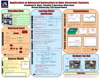
1. Real System + - Model Sensitivity Equations Real System Q Specify + e2 } e - + e1 - + - Form S(t) + - Use to continuously update Coefficients in model and Sensitivity equations - - Application of Advanced Automation in Opto-Electronic Systems Shubham K. Bhat, Timothy P. Kurzweg, Allon Guez Drexel University, ECE Department Introduction Learning Model Simulations Identification Automation is the key to high volume, low cost, and high consistency manufacturing ensuring performance, reliability, and quality. Noise, an external disturbance, inaccurate modeling could lead to deviation from the actual values. • No standard for OE packaging and assembly automation. • Misalignment is common between optical and geometric axes. • Packaging is critical to success or failure of optical microsystems. • 60-80 % cost of optical component/system is in packaging. MOTIVATION • Activated at a lower sampling frequency. • Specific and appropriate tasks. • Provides opportunities for the system to improve upon its power model. • Adjust the accuracy on the basis of “experienced evidence.” PROTOTYPE NEED FOR LEARNING Learning Identification Implementation 4 Piecewise Linear segments “+” represents the initial guesses of the plant model. “o” represents the final model (obtained using the learning algorithm). “-” represents the actual plant model. “o” represents the actual plant response. Other colored solid lines show how the actual slopes and intercepts are tracked from the initial guess. Model Based Control Correction toModel Parameter Step 1: Assume system to be described as , where y is the output, u is the input and is the vector of all unknown parameters. Learning Algorithm Model Parameter Adjustment FEED - FORWARD Set Point=Xo Assembly Alignment Task Parameters Visual Inspect and Manual Alignment Step 2: A mathematical model with the same form, with different parameter values is used as a learning model such that Optical Power Propagation Model AlGORITHM Edge Emitting Laser Coupled To a Fiber Near Field Coupling Piecewise Linear segments {Xk}, {Pk} Step 3: The output error vector, e , is defined as . Initialization Loop Move to set point (Xo) Measure Power (Po) Aperture = 20um x 20um Fiber Core = 4um Propagation Distance = 10um • ADVANTAGES: • Support for Multi-modal functions • Technique is fast • Cost-efficient Step 4: Manipulate such that the output is equal to zero. Step5: Itfollows that and BACKGROUND FIBER COUPLING Off the shelf Motion Control (PID) (Servo Loop) We present a system with two unknowns exhibiting input-output differential equation Stop motion Fix Alignment ( a and K are unknown ) The variables u, y, and are to be measured Step 1: { } and EXAMPLE { Assume estimated model and } Step 2: Learning Loop of PWL segment Learning Identification of two unknown variables PLANT RESPONSE INVERSE MODEL For the first segment, assuming a unity gain Pr(s) Pd(s) R(s) Kp E(s) + where , a and K have initial estimates of 0.1 and 4 and Step 3: The Sensitivity coefficients are contained in + + Desired Power - Received Power a and K have actual values of 1.44 and 5.23 FEEDBACK LOOP FEEDFORWARD LOOP Tracking parameter (e) is 0.08. Kp Accurate Plant and Inverse Model is the key to the success of Model Based Control. Hardware Test-Bed BLOCK DIAGRAM Inverse Model Receiver Fiber Power Meter Source (Laser) Power meter Test fiber • Required for Feed Forward Model. • Numerical Power models typically are non-invertible. • Zeros on the right half plane make the system unstable. • Excess of poles over zeros of Power distribution is non-monotonic (no 1-1 mapping). • Find “equivalent” set of monotonic functions. WHY? The learning model adjustment scheme consists of assuming initial values for , adjoining the sensitivity equations to the model equations and using . PID controller Inside the PC Sensitivity matrix S is given by • Decompose complex waveform into Piece-Wise Linear (PWL) Segments. • Each segment valid in specified region. • Find an inverse model for each segment. Break-out 60 Criteria for choosing e Linear Motor X-Y Amplifiers Aperture Encoder Interpolator HOW? If e is too large, the schemes will diverge. If e is too small, then will approach very slowly. Publications Selection of a suitable e and the weighting matrix Q are determined by a trial and error process. • Shubham K. Bhat, T.P.Kurzweg, Allon Guez.” Simulation and Experimental Verification of Model Based Opto-Electronic Packaging Automation”, Photonics East Conference, Philadelphia, October 26-28, 2004. • Shubham K. Bhat, T.P.Kurzweg, Allon Guez, “Advanced Packaging Automation for Opto-Electronic Systems”, IEEE Lightwave Conference, New York, October 2004 . • T.P. Kurzweg, A. Guez, S.K. Bhat, "Model Based Opto-Electronic Packaging Automation," IEEE Journal of Special Topics in Quantum Electronics, Vol.10, No. 3, May/June 2004, pp.445-454. • Shubham K. Bhat, T.P.Kurzweg, Allon Guez, “Improved Performance in Optical Communication System through Advanced Automation”, IEEE Sarnoff Symposium, April 2004.