Chapter 5 Sampling and Statistics
This chapter provides a comprehensive overview of sampling and statistical methods essential for estimating unknown parameters and formulating hypothesis tests. It discusses random variables, statistics, order statistics, and confidence intervals, with an emphasis on sampling techniques (with and without replacement). The text explores the estimation of parameters through sample data and highlights the significance of the central limit theorem in constructing confidence intervals. Additionally, the concept of hypothesis testing, including the definitions of null and alternative hypotheses, is introduced, along with the potential errors involved in decision-making.

Chapter 5 Sampling and Statistics
E N D
Presentation Transcript
Chapter 5Sampling and Statistics Math 6203 Fall 2009 Instructor: AyonaChatterjee
5.1 Sampling and Statistics • Typical statistical problem: • We have a random variable X with pdf f(x) or pmf p(x) unknown. • Either f(x) and p(x) are completely unknown. • Or the form of f(x) or p(x) is known down to the parameter θ, where θ may be a vector. • Here we will consider the second option. • Example: X has an exponential distribution with θ unknown.
Since θ is unknown, we want to estimate it. • Estimation is based on a sample. • We will formalize the sampling plan: • Sampling with replacement. • Each draw is independent and X’s have the same distribution. • Sampling without replacement. • Each draw is not independent but X’s still have the same distribution.
Random Sample • The random variables X1, X2, …., Xn constitute a random sample on the random variable X if they are independent and each has the same distribution as X. We will abbreviate this by saying that X1, X2, …., Xnare iid; i.e. independent and identically distributed. • The joint pdf can be given as
Statistic • Suppose the n random variables X1, X2, …., Xn constitute a sample from the distribution of a random variable X. Then any function T=T(X1, X2, …., Xn) of the sample is called a statistic. • A statistic, T=T(X1, X2, …., Xn), may convey information about the unknown parameter θ. We call the statistics a point estimator of θ.
Notation • Let X1 , X2, ….Xn denote a random sample from a distribution of the continuous type having a pdf f(x) that has a support S = (a, b), where -∞≤ a< x< b ≤ ∞. Let Y1 be the smallest of these Xi, Y2 the next Xi in order of magnitude,…., and Yn the largest of the Xi. That is Y1 < Y2 < …<Yn represent X1 , X2, ….Xn, when the latter is arranged in ascending order of magnitude. We call Yi the ith order statistic of the random sample X1 , X2, ….Xn.
Theorem 5.2.1 • Let Y1 < Y2 < …<Yn denote the n order statistics based on the random sample X1 , X2, ….Xn from a continuous distribution with pdf f(x) and support (a,b). Then the joint pdf of Y1 , Y2, ….Yn is given by,
Note • The joint pdf of any two order statistics, say • Yi < Yj can be written as
Note • Yn - Y1 is called the range of the random sample. • (Y1 + Yn)/2 is called the mid-range • If n is odd then Y(n+1)/2 is called the median of the random sample
The Statistical Problem • We have a random variable X with density f(x,θ), where θ is unknown and belongs to the family of parameters Ω. • We estimate θ with some statistics T, where T is a function of the random sample X1 , X2, ….Xn. • It is unlikely that value of T gives the true value of θ. • If T has a continuous distribution then P(T= θ)=0. • What is needed is an estimate of the error of estimation. • By how much did we miss θ?
Central Limit Theorem • Let θ0 denote the true, unknown value of the parameter θ. Suppose T is an estimator of θ such that • Assume that σT2 is known.
Note • When σ is unknown we use s(sample standard deviation) to estimate it. • We have a similar interval as obtained before with the σ replaced with st. • Note t is the value of the statistic T.
Confidence Interval for Mean μ • Let X1 , X2, ….Xn be a random sample from the distribution with unknown mean μ and unknown standard deviation σ.
Note • We can find confidence intervals for any confidence level. • Let Zα/2 as the upper α/2 quantile of a standard normal variable. • Then the approximate (1- α)100% confidence interval for θ0 is
Confidence Interval for Proportions • Let X be a Bernoulli random variable with probability of success p. • Let X1 , X2, ….Xn be a random sample from the distribution of X. • Then the approximate (1- α)100% confidence interval for p is
Introduction • Our interest centers on a random variable X which has density function f(x,θ), where θ belongs to Ω. • Due to theory or preliminary experiment, suppose we believe that
The hypothesis H0 is referred to as the null hypothesis while H1 is referred to as the alternative hypothesis. • The null hypothesis represents ‘no change’. • The alternative hypothesis is referred to the as research worker’s hypothesis.
Error in Hypothesis Testing • The decision rule to take H0 or H1 is based on a sample X1 , X2, ….Xn from the distribution of X and hence the decision could be wrong.
The goal is to select a critical region from all possible critical regions which minimizes the probabilities of these errors. • In general this is not possible, the probabilities of these errors have a see-saw effect. • Example if the critical region is Φ, then we would never reject the null so the probability of type I error would be zero but then probability of type II error would be 1. • Type I error is considered the worse of the two.
Critical Region • We fix the probability of type I error and we try and select a critical region that minimizes type II error. • We saw critical region C is of size α if • Over all critical regions of size α, we want to consider critical regions which have lower probabilities of Type II error.
We want to maximize • The probability on the right hand side is called the power of the test at θ. • It is the probability that the test detects the alternative θ when θ belongs to w1 is the true parameter. • So maximizing power is the same as minimizing Type II error.
Power of a test • We define the power function of a critical region to be • Hence given two critical regions C1 and C2 which are both of size α, C1 is better than C2 if
Note • Hypothesis of the form H0 : p = p0 is called simple hypothesis. • Hypothesis of the form H1 : p < p0 is called a composite hypothesis. • Also remember α is called the significance level of the test associated with that critical region.
Introduction • Originally proposed by Karl Pearson in 1900 • Used to check for goodness of fit and independence.
Goodness of fit test • Consider the simple hypothesis • H0 : p1 =p10 , p2 =p20 , …, pk-1 =pk-1,0 • If the hypothesis H0 is true, the random variable • Has an approximate chi-square distribution with k-1 degrees of freedom.
Test for Independence • Let the result of a random experiment be classified by two attributes. • Let Ai denote the outcomes of the first kind and Bj denote the outcomes for the second kind. • Let pij = P(Ai Bj) • The random experiment is said to be repeated n independent times and Xij will denote the frequencies of an event in Ai Bj
The random variable • Has an approximate chi-square distribution with (a-1)(b-1) degrees of freedom provided n is large.